Project 1 - Parsing NASA thermodynamic data
Aim:
In this project, we are going to obtain a set of 14 coefficients from NASA thermodynamic data file and use them to calculate the enthalpy, entropy and specific heat of a set of 53 species. We will also be making plots showing the variation of enthalpy, entropy and specific heat with temperature for each of those species. In the end, we will be calculating their molecular masses.
To calculate the enthalpy, entropy and specific heat, we will be using the following equation:

where we will be using the first 7 coefficients for high temperature ranges and remaining coefficients for low temperature ranges.
Code:
clear all
close all
clc

f1= fopen('THERMO.dat','r')
line1 = fgetl(f1);
line2 = fgetl(f1);
A = strsplit(line2,' ');
%extracting global temperature ranges
global_low_temperature = str2num(A{2});
global_mid_temperature = str2num(A{3});
global_high_temperature = str2num(A{4});

%skipping the next three lines
fgetl(f1);
fgetl(f1);
fgetl(f1);

%capturing data of the 53 different species
for i = 1:53
    line_i = fgetl(f1);
    %finding local temperature ranges
    t = strfind(line_i,'.');
    %t = 52 62 72
    tl = line_i(t(1)-3:t(1)+3);
    t_low = str2num(tl);
    th = line_i(t(2)-4:t(2)+4);
    t_high = str2num(th);
    tm = line_i(t(3)-4:t(3)+4);
    t_mid = str2num(tm);

    species_name = line_i(1:6);

    %obtaining the coefficients from first line
    cline1 = fgetl(f1);
    c = strfind(cline1,'E');
    coeff1 = cline1(c(1)-10:c(1)+3);
    c1 = str2num(coeff1);
    coeff2 = cline1(c(2)-11:c(2)+3);
    c2 = str2num(coeff2);
    coeff3 = cline1(c(3)-11:c(3)+3);
    c3 = str2num(coeff3);
    coeff4 = cline1(c(4)-11:c(4)+3);
    c4 = str2num(coeff4);
    coeff5 = cline1(c(5)-11:c(5)+3);
    c5 = str2num(coeff5);

    %obtaining the coefficients from second line
    cline2 = fgetl(f1);
    d = strfind(cline2,'E');
    coeff6 = cline2(d(1)-10:d(1)+3);
    c6 = str2num(coeff6);
    coeff7 = cline2(d(2)-10:d(2)+3);
    c7 = str2num(coeff7);
    coeff8 = cline2(d(3)-10:d(3)+3);
    c8 = str2num(coeff8);
    coeff9 = cline2(d(4)-10:d(4)+3);
    c9 = str2num(coeff9);
    coeff10 = cline2(d(5)-10:d(5)+3);
    c10 = str2num(coeff10);

    %obtaining the coefficients from third line
    cline3 = fgetl(f1);
    e = strfind(cline3,'E');
    coeff11 = cline3(e(1)-10:e(1)+3);
    c11 = str2num(coeff11);
    coeff12 = cline3(e(2)-10:e(2)+3);
    c12 = str2num(coeff12);
    coeff13 = cline3(e(3)-10:e(3)+3);
    c13 = str2num(coeff13);
    coeff14 = cline3(e(4)-10:e(4)+3);
    c14 = str2num(coeff14);

    %splitting our local temperature range into 100 values
    T = linspace(t_low, t_high, 100);
    %Universal gas constant
    R = 8.314; %in J/mol-k
    for  j = 1:length(T)
        if T(j)<t_mid %we will be using the low temperature coefficients
            cp = (c8+(c9.*T)+(c10.*T.^2)+(c11.*T.^3)+(c12.*T.^4))* R;
            H = (c8 + ((c9.*T)./2)+ ((c10.*T.^2)/3)+((c11.*T.^3)/4)+((c12.*T.^4)/5)+(c13./T)).*T.*R;
            S = (c8*log(T) + c9.*T + c10.*(T.^2)/2 + c11.*(T.^3)/3 + c12.*(T.^4)/4 + c14).*R;
        else
            %we will be using the high temperature coefficients
            cp = (c1+(c2.*T)+(c3.*T.^2)+(c4.*T.^3)+(c5.*T.^4)) * R;
            H = (c1 + ((c2.*T)./2)+ ((c3.*T.^2)/3)+((c4.*T.^3)/4)+((c5.*T.^4)/5)+(c6./T)).*T.*R;
            S = (c1.*log(T) + c2.*T + c3.*(T.^2)/2 + c4.*(T.^3)/3 + c5.*(T.^4)/4 + c7).*R;
        end
    end

        %specifying and changing the directory
        directory = (['C:\Users\mriga\Desktop\MATLAB\File Parsing\Species\',species_name]);
        cd(directory)


        %plotting and saving temperature vs specific heat graph
        figure(1)
        plot(T,cp,'color','r');
        xlabel('Temperature')
        ylabel('Specific Heat');
        title(species_name);
        saveas(1,'specific heat');

        %plotting and saving temperature vs enthalpy graph
        figure(2)
        plot(T,H,'color','b');
        xlabel('Temperature');
        ylabel('Enthalpy');
        title(species_name);
        saveas(2,'Enthalpy');

        %plotting and saving temperature vs entropy graph
        figure(3)
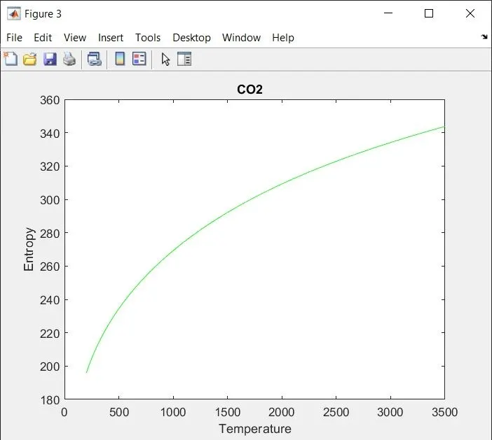
        plot(T,S,'color','g');
        xlabel('Temperature');
        ylabel('Entropy');
        title(species_name);
        saveas(3,'Entropy');


        cd('C:\Users\mriga\Desktop\MATLAB\File Parsing\')

        %calculating the molecular mass of each species
        species_name
        elements = ['H','C','N','O','A'];
        at_wt = [1 12 14 16 40];
        mm = 0;
        for i = 1:length(species_name)
            for j = 1:length(elements)
                 %comparing the two strings to obtain atomic weight of a
                 %particular element
                 if strcmp(species_name(i),elements(j))
                    mm = mm + at_wt(j);
                    x = j;
                 end
            end
            %checking if there are more than one atoms of a particular
            %element and improvising our calculation accordingly
            y = str2num(species_name(i));
            if y>1
                mm = mm + at_wt(x)*(y-1);
            end
        end
    %molecular mass obtained
    mm
end
Explanation of the code:
1. To open the data file and to read its contents, we will be using the 'fopen' and 'fgetl' commands respectively.
2. To obtain the global temperatures, we will use the split the low, medium and high temperature values using 'strsplit' command and assign these to variables accordingly.
3. Now, we will initiate a 'for-loop' that runs 53 times in order to obtain the local temperatures and the coefficients of all the 53 species. In each loop, the first line will give us the temperature data and the second, third and fourth line will gives us the coefficients.
4. Since, these values will be stored initially as a string, we will use the 'str2num' command to convert them into numerical format.
5. We will use 'linspace' command to split the local temperature range into a 100 values and then using the equations provided we will calculate the enthalpy, entropy and specific heat.
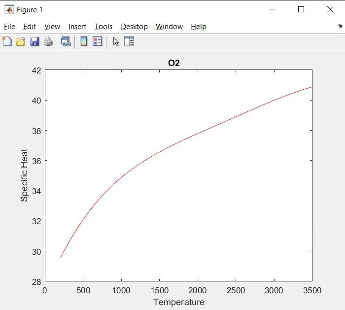
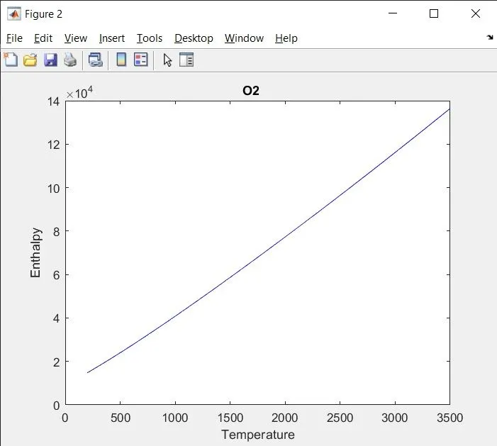
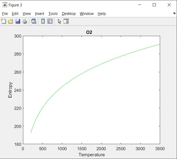
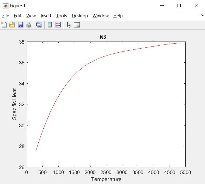
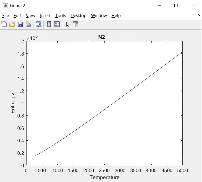
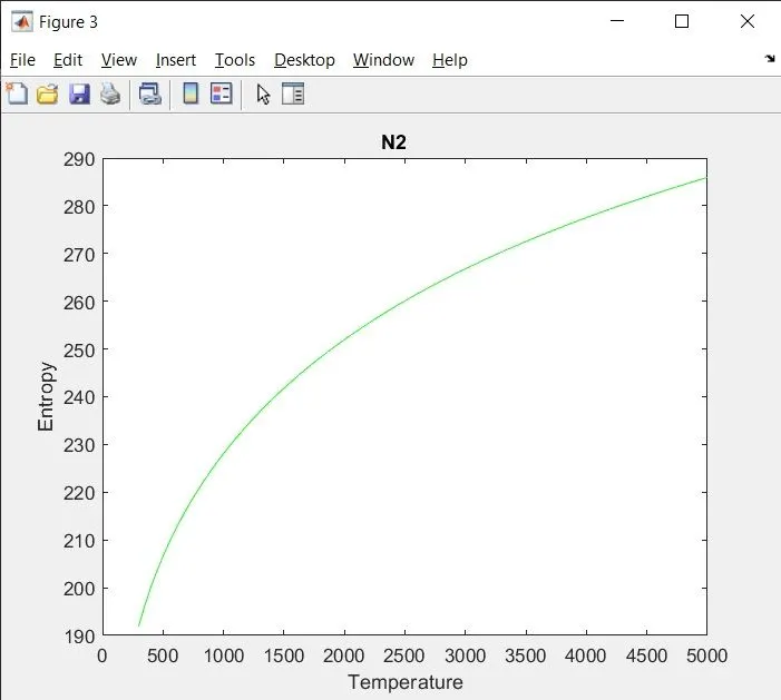
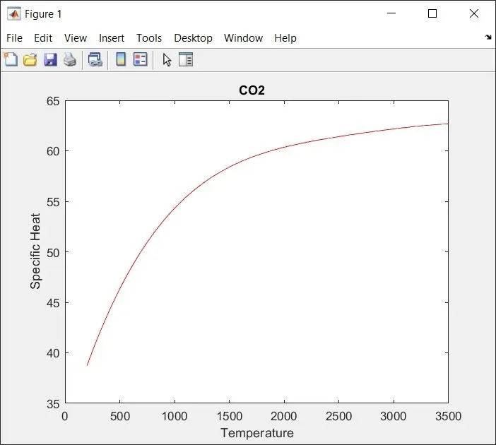
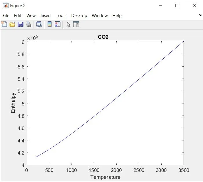
6. We will then plot three graphs, showing the variation of enthalpy, entropy and specific heat with temerature and save them using 'saveas' command. We need to specify the directory before saving the plots.
7. Finally, to calculate the molecular mass of the species we will define two strings namely 'elements' and 'at_wt' containing all the elements and their respective atomic masses respectively. The calculations involved would then calculate the molecular mass of the species based on the elements present and the number of atoms present of each element.
Results:
1. Plots of O2
2. Plots of N2
3. Plots of CO2
4. Folder containing the plots