Week-4 Challenge WOT Condition Part-2

Q1:

When we go inside the Electric Plant and inside the motor block we have two kinds of models representing the motor-generator/Engine inside the EV:

• Mapped Motor-Generator/Engine model[Global Based Model]
• Dynamic Model[Real-Time based]

The differences between the two are as follows:

1. The Mapped model also called the static model consists of a lookup table with the motor/generator/Engine data. We can map the data to this file and can simulate the model. In the Dynamic model, however, we have the actual components of a motor/generator/Engine along with the motor drive, inverter, the spark plug type, and so on.
2. The mapped model will run faster than the dynamic model.
3. The mapped model is easier to implement than the dynamic model.
4. However, the mapped model is simpler and faster to implement and run, the dynamic model will give a more accurate result of the simulation and would provide more analysis options.

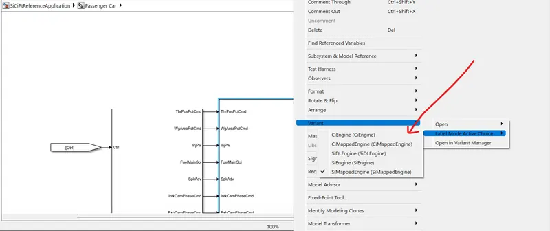
To switch between these two models, we need to right-click the model's subsystem where the engine or motor is positioned.

To do this first go to the variant manager, right-click on the model, choose the variant type you want to apply, and then make the label mode choice active by clicking on the option.

Q2:

In the model fuel flow/fuel efficiency calculations, the following parameters are considered:

1. Vehicle Velocity
2. Fuel Flow volume
3. If the vehicle is BEV or HEV, the Battery Power being consumed will also affect the fuel efficiency calculation.

Shown below is a Reference Application for a SI, CI engine-based vehicle.

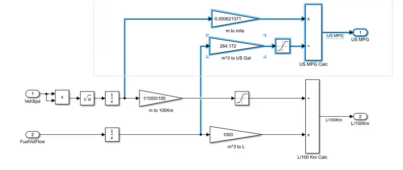
We can see that the US MPG calculation takes place in 2 main steps. First, the m^3 is converted to gallon which is the volume of the fuel flowing into the engine while it drives the vehicle. The vehicle speed is integrated to find the displacement(or distance traveled of the vehicle) after which the meters traveled are converted to miles. This gives us the final miles/gallon ratio also known as the equivalent MPG. Note that in the case of vehicles with both fuel injection as well as battery power, the MPG is actually the equivalent MPG and in most cases provides very high numbers of fuel economy as compared to standard engine-driven vehicles.

Q3:

The original WOT condition with default settings for the HEV Application file gives us the following graph:

Runtime= 30 seconds

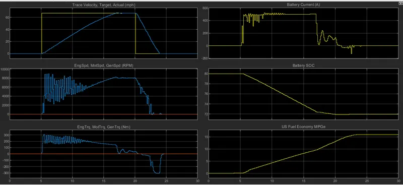
(Fig A: Fuel Efficiency and Performance Plots)

Now the wind velocity and grade are modified to 3 and 7 units respectively:

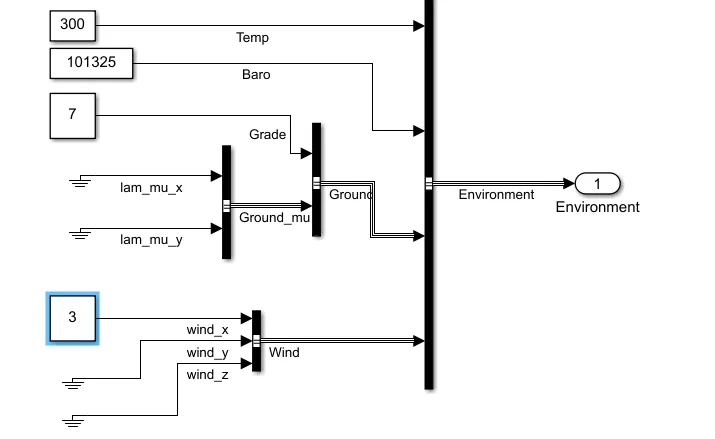
The HEV powertrain model is simulated again keeping everything exactly the same and the following results are obtained as below:

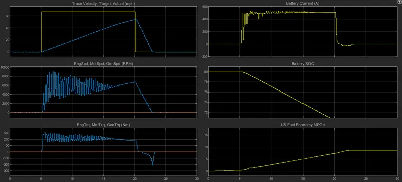
(Fig B: Fuel Efficiency and Performance Plots)

The Pure EV powertrain model is simulated again keeping everything exactly the same and the following results are obtained as below:

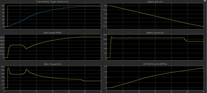
(Fig C: Fuel Efficiency and Performance Plots)

A comparison of the two different results is done below-

Plot	Figure A	Figure B
Plot 1 Trace Velocity	The actual speed given in blue tries to follow the given set target speed in yellow and achieves it after initially lagging.	In the actual curve, the blue line tries to follow the drive cycle values but cannot due to the grade of the road.
Plot 2 Eng, Motor, and Generator Speeds	The curve is almost the same but has a smoother slope.	The slope here is much steeper as due to the grade, the load on the engine has increased significantly.
Plot 3 Engine, motor, and generator torques	No visible differences	-
Plot 4 Battery Current	The fluctuation of the battery current in the initial part eventually smoothens out and the battery current demand reduces drastically.	The battery current fluctuations at higher levels do not smoothen to a constant value till a later time and moreover, the battery current demand doesn't reduce immediately.
Plot 5 Battery SOC	Battery SOC drops gradually	Battery SOC drops suddenly due to high power demand considering the grade.
Plot 6 US Economy Miles Per Gallon	Comparatively, high MPG is achieved.	Lower MPG due to the grade effect.