Week-4 Challenge WOT Condition Part-2
1. Mapped Model: Here, the model uses a predefined set of values such as a look table to characterize the performance. This table provided the overall characteristics with respect to engine, motor, or generator. This is also known as a static model and it takes less time to simulate as it does not involve real-time outputs from the subsystem.
Dynamic Model: Here, the model will split the behavior of the component into particular characteristics into lower-level components which adds the dynamic effect to the system. This takes more time compared to the mapped model. This model involves real-time outputs from different subsystems hence the results are more accurate in this case.
2. EV Reference Model from MATLAB is used to understand how miles per gallon can be calculated. The below figure shows the EV model reference which is a closed-loop system as the velocity is taken as feedback and compared with the drive cycle hence also called a forward-facing model.
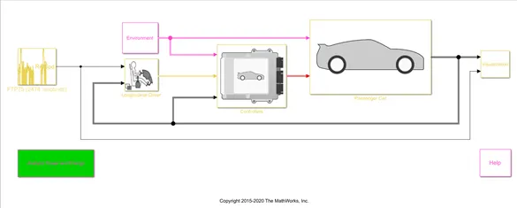
This model consists of a drive cycle FTP75 based which is compared with the actual velocity of the vehicle, the error is calibrated by the driver. The controller controls based on the driver's wish and the environmental forces acting on the vehicle. In the Visualisation, we can get the conversion calculation for miles per gallon in the system Performance Calculation.
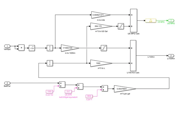
The vehicle speed is squared with a product block to make sure the speed is always positive. This value is square rooted to get the speed of the vehicle. Integration of speed gives us distance. This distance is a converter from meters to 100 km with the help of a gain block which is passed through a saturation block to get the value in km.
The battery power is converted from W to KW to US EPA kWh per hour with the help of a few calculations which finally gives us m3 per gallon which is integrated and converted to liters (L). Now liters are divided by 100km using a product block to get the L/100km value.
The distance in m which is an integrated value of speed is converted to miles is divided by cubic meters to get miles per gallon (US MPG) as shown in the figure below.
3. HEV ReferenceApplication is run in MATLAB Simulink. The model is shown in the figure below.
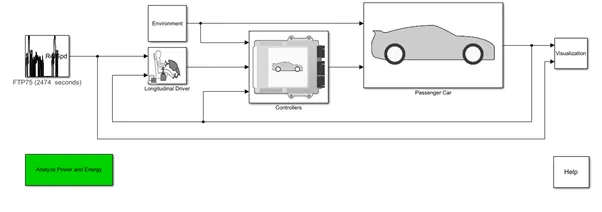
This HEV Reference Model is Run with WOT drive cycle using MATLAB Simulink is shown in the figure below. 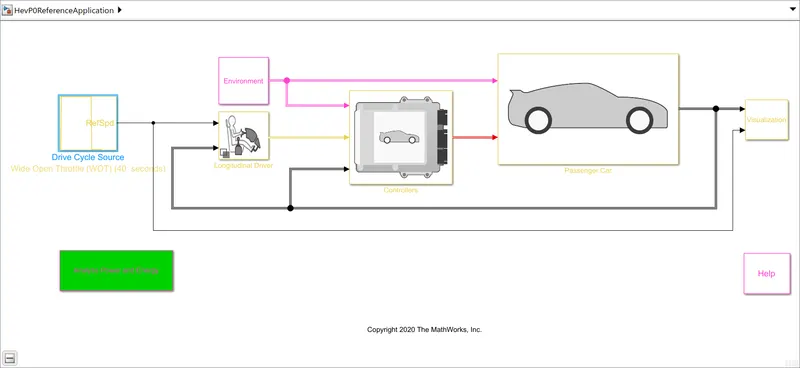
the Wide Open Throttle Drive Cycle is given by
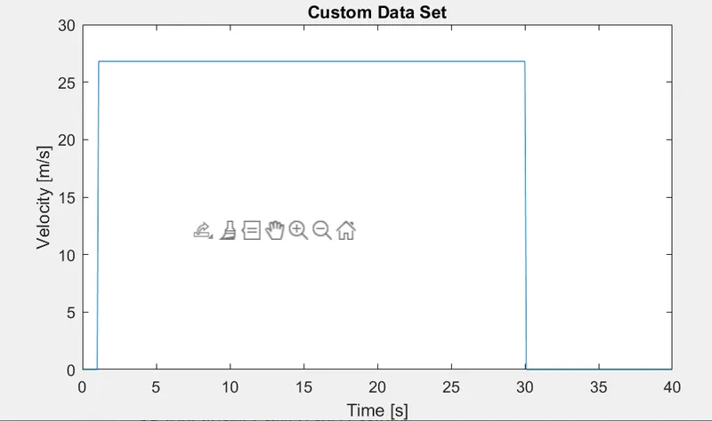
the results can be as shown in the figure.
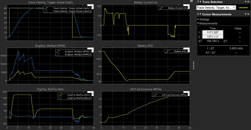
It can be seen from the scope of the results that Actual velocity does not follow the WOT drive cycle, as there cannot be a sudden acceleration in a practical scenario. There is gradual acceleration until the maximum speed is reached. The engine and motor speed required to reach max acceleration is high compared to theoretical conditions. The engine and motor torque is not high in the expected calculation, as there will not be any sudden acceleration. The battery current required is high when there is acceleration, constant when there is no change in speed, the battery charges during deceleration. The percentage of SOC of the vehicle reduces due to max acceleration, remains constant for constant speed, and later increases as the battery charges due to reverse current during deceleration. The fuel economy miles per gallon increases at the end of WOT drive cycle test which can be inferred from the results.
4. Comparing the powertrains of pure electric and hybrid power train.
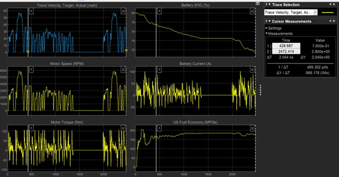
Fig1: Performance parameters of Pure Electric Powertrain
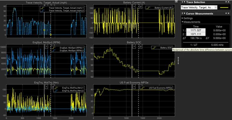
Fig2: Performance parameters of Hybrid Electric PowerTrain
It can be seen from both the figures that, both EV and HEV powertrains are run with FTP75 drive cycle.
The actual velocity follows the reference velocity in both cases.
The motor speed changes as per the drive cycle in the case of EV whereas, the engine rpm and motor rpm changes drastically compared to reference speed in HEV.
The torque varies as per acceleration and deceleration in the case of EV, whereas the torque required by engine and motor is less compared to reference in HEV due to hybrid powertrains in HEV application.
The SOC of the battery decreases during acceleration is constant during idle and increases during deceleration in both cases.
The variation of battery current varies with acceleration or deceleration of the vehicle in both cases.
The fuel economy increases up to 200 and 40 in EV and HEV respectively as inferred from the graph.