Project

AIM:

To analyze and carry out a system-level Simulation of an All-Terrain-Vehicle using the Simulink model.

INTRODUCTION:

An all-terrain vehicle (ATV) as shown in Fig1 is also known as a light utility vehicle (LUV), a quad bike, or simply a quad, as defined by the American National Standards Institute(ANSI); is a vehicle that travels on low-pressure tires, with a seat that is straddled by the operator, along with handlebars for steering control. As the name implies, it is designed to handle a wider variety of terrain than most other vehicles.

By the current ANSI definition, ATVs are intended for use by a single operator, although some companies have developed ATVs intended for use by the operator and one passenger. These ATVs are referred to as tandem ATVs.The rider sits on and operates these vehicles like a motorcycle, but the extra wheels give more stability at slower speeds. Although most are equipped with three or four wheels, six-wheel models exist for specialized applications.

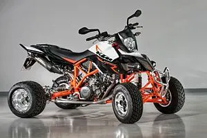
Fig1: A KTM Quad 990 All-Terrain-Vehicle.

REVIEW OF BAJA SAE COMPETITION OF ALL-TERRAIN-VEHICLE (as given in the link)

Baja SAE is a Collegiate Design Series competition run by the Society of Automotive Engineers International (SAE International). Teams of students from universities all over the world design and build small off-road cars. The cars all have engines of the same specifications. As of 2018, the engine has been an unmodified Briggs & Stratton Model 19 Vanguard engine single-cylinder with a displacement of 305cc and a power output of approximately 10 bhp (7.5 kW).

The goal in Baja SAE racing is to design, build and race off-road vehicles that can withstand the harshest elements of rough terrain. Each year as many as 141 Baja cars are entered in the Baja SAE events across the US and around the world.

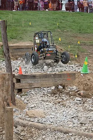
Fig2: Picture of the Purdue University Northwest vehicle navigating a jump at the 2019 Baja Midwest event at Tennessee Tech University.

Courtesy: Wikipedia

BAJA ATV MODEL WITHOUT DASHBOARD

COMPONENTS OF A BAJA ATV

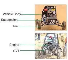
Fig 3: Components of BAJA ATV.

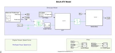
Fig 4: Simulink Model of a BAJA ATV.

1. Engine:

The Generic Engine Block represents a system-level model of spark-ignition and diesel engines suitable for use at the initial stages of modeling when only the basic parameters are available. The throttle input signal T lies between zero and one and specifies the torque demanded from the engine as a fraction of the maximum possible torque. If the engine speed falls below the Stall speed, the engine torque is blended to zero. If the engine speed exceeds the maximum speed, the simulation stops and issues an error message.

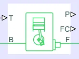
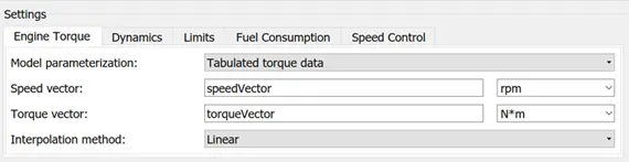
Fig 5: Generic Engine Block and settings

The speed vector and torque vector values are taken from the tabulated data in the workspace.

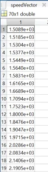
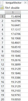
Fig 6: Speed and torque vector values for Generic Engine Block

Connections F and B are mechanical rotational conserving ports associated with the engine crankshaft and engine block, respectively.

Connections P and FC are physical signal output ports through which engine power and fuel consumption rate are reported.

2. Simple Gear:

Represents a fixed-ratio gear or gearbox. No inertia or compliance is modeled in this block. This is used mostly in an internal combustion engine to drive the wheels. They run at high speed and subsequent speed goes to wheels when connected through a gear. With the help of a transmission speed can be reduced and torque can be increased.

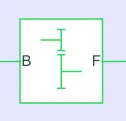
Connections B (base) and F (follower) are mechanical rotational conserving ports.

Fig 7: Simple Gear Block and Settings

3. CVT block:

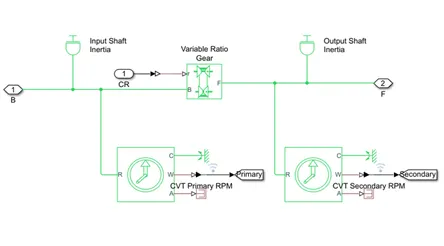
Fig 8: CVT Transmission Subsystem

A CVT transmission, or continuously variable transmission, seamlessly changes through an unending range of effective gear ratios while you drive, whereas other kinds of mechanical transmissions offer a fixed number of gear ratios and have hard shifts between each.CVT transmission systems are also known as single-speed, shiftless, and step-less transmissions. The shiftless nature of a CVT offers unparalleled flexibility that maintains constant angular velocity regardless of output speed. Additionally, a continuously variable transmission makes accelerating smooth and offers enhanced fuel economy.

This system consists of cones at each pulley connected via a chain belt. The cones can move to increase or decrease the belt diameter to change gear ratios, allow for quick shifting into the needed ratio for increased power, and boost fuel economy.

One pulley in the CVT is connected to the engine and the other directs power to the wheels. The width of these pulleys changes based on the needed power; as one gets larger, the other gets smaller. This allows a CVT to deliver strong and seamless acceleration.

Though there are no gears in a CVT, some simulate a more traditional changing of gears. In these transmissions, the belt-and-pulley system is designed to move to preset points by using a traditional shift lever or paddle shifters on the steering wheel.

4. Vehicle body:

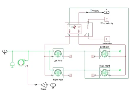
Fig 9: Vehicle Body Subsystem

The vehicle body is designed to overcome the different forces acting on it. The force that enables the vehicle to propel forward is called Tractive Effort. This force is due to the contact between the wheel of the vehicle on the road.

According to Newton’s Law of Motion,

Vehicle Acceleration is given by,

Where

The resistance forces encountered by a vehicle are:

• Rolling resistance force
• Aerodynamic drag
• Gradient resistance / Uphill drag

1. Rolling Resistance force (Fr):

Rolling resistance is the combination of forces that work against the forward motion of the vehicle. The weight of the vehicle, gravity and inertia, the amount of friction between the tires and the road surface, and air drag all play a part. When you coast a vehicle, rolling resistance is what slows down the vehicle. The more rolling resistance, the more power it takes to propel a vehicle.

When a vehicle is moving on a

• Hard surface: The rolling resistance is primarily due to hysteresis in tire materials. This hysteresis is caused due to deflection/deformation of the skeleton of the tire which causes the asymmetric distribution of the ground reaction force.
• Soft surface: Here, the rolling resistance is primarily due to the deformation of ground surfaces. When a vehicle moves this deformation causes the pressure in the leading half of the tire to be more than the trailing half. Due to which even if the total load on the vehicle is constant, there is an unequal distribution of forces.

Rolling resistance force (N) is given by

Fr = m *g*fr*cos⍺

Where m – mass (kg)

g – force due to gravity (m/s²)

fr – rolling resistance coefficient

⍺ - gradient angle

2. Aerodynamic Drag (Fw):

Any vehicle traveling at a speed in air encounters a force resisting its motion. This consists of two components:

• Shape/ Pressure drag: The forward motion of the vehicle pushes the sir in front of it, but the air cannot instantaneously move out of the way which results in the creation of a high-pressure zone ahead of the vehicle. Also, a low-pressure region is created behind the vehicle as the air instantaneously fills the left space. This pressure difference induces a drag due to the shape of the car.
• Skin Friction Drag: Air molecules near the skin of the vehicle move at a speed equal to that of the vehicle while the air molecules far from the vehicle remain at rest. The molecules of air between these layers move at a wide range of speeds from zero to vehicle speed. This disturbance occurs due to the friction force which results in the second component of aerodynamic drag.

Aerodynamic Drag Force (N) is given by

Fw = 0.5*ƍ* Af* Cd*(V-Vw)²

Where ƍ – air density (kg/m³)

Af – Frontal area of the vehicle (m²)

Vw – Wind Velocity (m/s)

Cd – Drag coefficient

3. Gradient Force / Uphill Force(Fg):

When the vehicle travels uphill, a component of its weight works in a direction opposite to its motion. If some energy is not supplied to overcome this backward force, then the vehicle would slow down, stall and roll backward. If the vehicle is trading uphill at a slope of θ, then the weight of the vehicle, W has two components: one perpendicular to the road surface and the other along the road surface.

The gradient resistance (N) is given by:

Fg = M*g*sin⍺

Where m – mass (kg)

g – force due to gravity (m/s²)

⍺ - gradient angle (degrees)

Overall Tractive Effort is given by:

Ft = Fr + Fw + Fg + Fa

Where Fr – Rolling resistance force (N)

Fw – aerodynamic drag Force (N )

Fg – gradient force (N)

Fa – acceleration force (N)

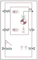
Fig 10: Simscape Vehicle Body Block

Connection H is the mechanical translational conserving port associated with the horizontal motion of the vehicle body. The resulting traction motion developed by tires should be connected to this port.

Connections V, NF, and NR are physical signal output ports for vehicle velocity and front and rear normal wheel forces, respectively. Wheel forces are considered positive if acting downwards.

Connections W and beta are physical signal input ports corresponding to headwind speed and road inclination angle, respectively.

5. Tire:

Represents the longitudinal behavior of a highway tire characterized by the tire Magic Formula. The block is built from Tire-Road Interaction (Magic Formula) and Simscape Foundation Library Wheel and Axle blocks. Optionally, the effects of tire inertia, stiffness, and damping can be included.

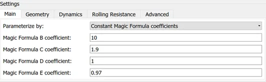
Fig 11: Tire Block and Settings

Connection A is the mechanical rotational conserving port for the wheel axle.

Connection H is the mechanical translational conserving port for the wheel hub through which the thrust developed by the tire is applied to the vehicle.

Connection N is a physical signal input port that applies the normal force acting on the tire. The force is considered positive if it acts downwards.

Connection S is a physical signal output port that reports the tire slip.

WORKING :

The input signals are generated using the signal builder block which is directly connected to the engine. A brake signal is also created with the signal builder block whose signal is given to the vehicle body. The generic Engine block is attached with a solver to run the simulation and gives an output speed that is achieved by the crankshaft output. This value is read from the RPM sensor i.e., a rotational motion sensor which gives the value of the engine output rpm.
This engine output rpm is given to the CVT to reduce the speed of the vehicle. A CVT ratio is created using a signal builder block and is provided to the CVT transmission block. The output speed is controlled by the CVT ratio as shown in fig 14 which is the input to a simple gear. This controlled speed acts as an input to the vehicle's body to accelerate the vehicle forward. The velocity at which the vehicle is propelling is read through a scope for further analysis.

The input given to the model in fig 4 is

- brake input is zero.

- throttle input is from 0.3 at t= 0 secs to 1 at t = 20secs and after.

The input signals are as shown in fig 12.

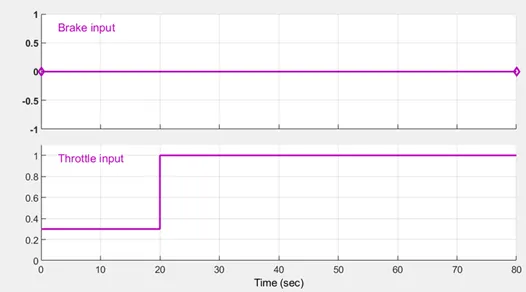
Fig 12: Brake and Throttle input to BAJA ATV.

It can be observed at the output plot that, as the throttle varies from 0.3 to 1 at t = 20secs, the velocity increases and reaches the maximum velocity as shown in fig 13.

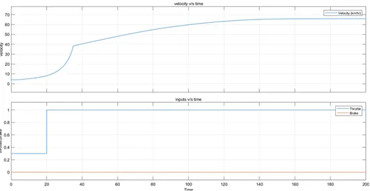
Fig 13: Output plot of BAJA ATV.

CVT gear ratio block:

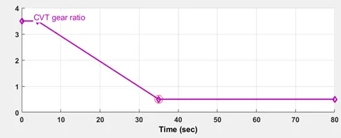
Fig 14:CVT gear ratio signal builder block.

Engine Sensor:

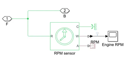
Fig 15: Engine Sensor Subsystem.

RESULTS:

Torque - Speed Plot:

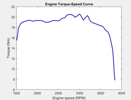
Fig 16: Input to the engine block to generate output rpm.

Fig 17: Output plot of BAJA ATV.

CVT Shaft Speed Plot:

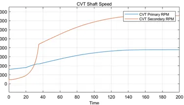
Fig 18: CVT primary and secondary rpm

Therefore, the BAJA All-Terrain Vehicle system’s Simulink model is analyzed, the results are observed and reported.

BAJA ATV MODEL WITH DASHBOARD

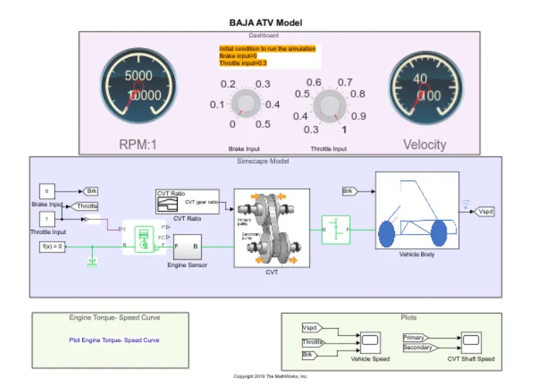
Fig 19: BAJA ATV Model with the dashboard.

The process of this model remains the same as the BAJA ATV model without a dashboard but the inputs throttle and break that were given by a signal builder block can be directly given by the user by tunning using the knob.

RESULTS:

CVT Reduced Speed Plot:

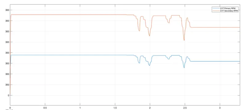
Fig 20: Reduced Speed plot.

The engine speed is reduced by controlling the CVT ratio.

Velocity Plot:

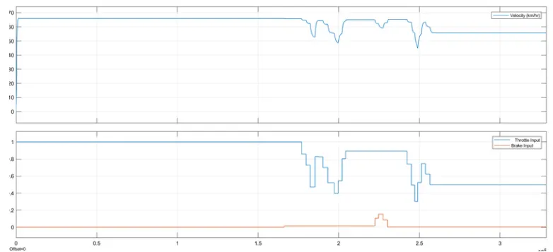
Fig 21: Velocity Plot:

It can be seen from fig 21 that there is acceleration and deceleration when throttle and brake are applied by the user.

BAJA ATV WITH LOOKUP TABLE

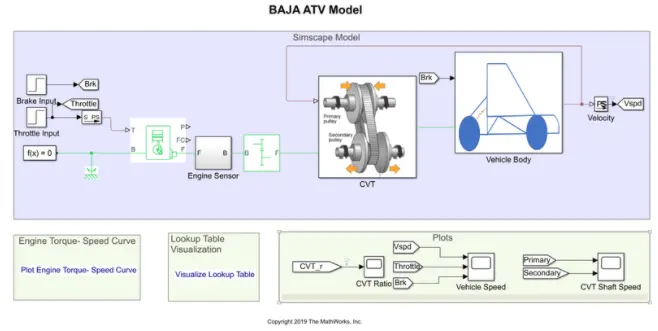
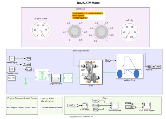
Fig 21: BAJA ATV Simulink Model with and without dashboard respectively and with the lookup table

The model is as shown in fig 21. Here, a input is given using a lookup table as shown in fig 23. The input is not generated using a signal builder block or manual input by the user. This lookup table data gives the relation between the CVT ratio and vehicle speed.

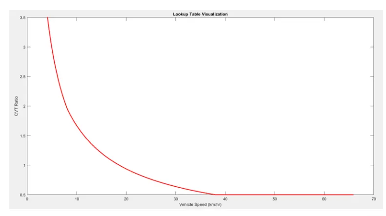
Fig 23: Lookup Table to set the inputs for the engine and CVT transmission

Therefore, BAJA ATV is analyzed based on different types of inputs. This study focuses on CVT transmission and shows the effect of CVT on the vehicle velocity with different types of Simulation Models of All-Terrain- Vehicles.