Week-4 Challenge WOT Condition Part-2

AIM:

• To understand the difference between Mapped & Dynamic model of engine, motor and generator, and procedure for changing model type
• To understand the calculation of miles per gallon & factors considered while modeling fuel flow
• To run the HEV Reference Application with WOT drive cycle & observe the effects of grade & wind velocity by changing the parameters from the environment block
• To run & compare simulated results of hybrid & pure electric powertrains.

OBJECTIVE:

• Study the mapped & dynamic models, their behavior, their advantages & disadvantages.
• Learn to change model types.
• Study the fuel flow model & equivalent calculation in miles per gallon.
• Study the effects of grade & wind velocity of HEVs.
• Compare the performance of pure EV & HEV under similar environmental conditions.

STUDY:

Understanding the difference between Mapped & Dynamic model of engine, motor and generator, and procedure for changing model type.

In the case of Mapped models, preassigned data is taken from a look-up table that has been predefined for the model and there are no real-time considerations. Due to the absence of real-time data, the simulation is faster but less accurate compared to the dynamic model. Mapped models are generally preferred when the input is unknown to us and the output can be obtained based upon the pre-defined data. Another important drawback of this model is that more data needs to be taken into account and assumptions need to be done.

E.g. Mapped engines represent macro engine behavior as a set of lookup tables (brake torque, fuel flow, air mass flow, exhaust temperature, efficiency, and emissions) as functions of commanded load and measured engine speed.

In the case of a Dynamic model, the final output is a result of the combination of outputs of several subsystems operating according to real-time inputs. These values which are fed as input to the subsystems, change with time, based upon the feedback from the previous results. The simulation for the dynamic model takes a longer time compared to mapped models due to the multiple simultaneous simulations under progress. However, the results, in this case, are more accurate due to the real-time output of subsystems being considered for the final output.

E.g. Dynamic engines decompose engine behavior into individual component models that account for engine dynamics, most notably intake airflow and turbocharger dynamics.

Steps to change model type:

1. Open the HEV Multimode Reference Application Model in MATLAB.
2. Double click and enter the “Passenger Car” sub-block, you’ll find Engine & Electric Plant block.
3. If you want to change the Engine Model.
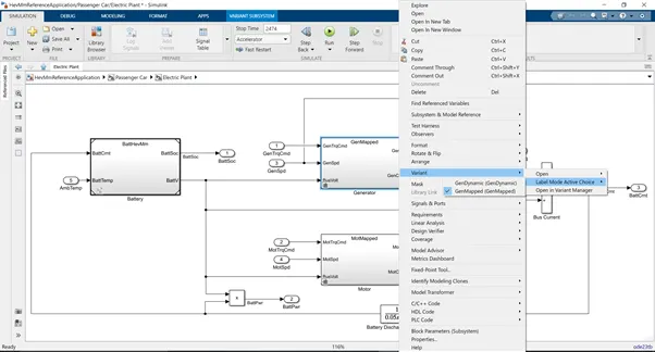
4. Select & right-click on the Engine block, a range of options will appear, select the “Variant” option, under the “Variant” option select the “Label Mode Active Choice” option and from there select the model you want to simulate with.
5. If you want to change the Motor/Generator variant, double click on the Electric Plant sub-block, you’ll find two different blocks inside, one for Motor & another for Generator.
6. If you want to change the Motor model, select & right-click on the Motor block, a range of options will appear, select the “Variant” option, under the “Variant” option select the “Label Mode Active Choice” option, and from there select the model you want to simulate with.
7. Likewise, if you want to change the Generator model, select & right-click on the Generator block, a range of options will appear, select the “Variant” option, under the “Variant” option select the “Label Mode Active Choice” option, and from there select the model you want to simulate with.

An example is shown below:

2. Understanding the calculation of miles per gallon & factors considered while modeling fuel flow.

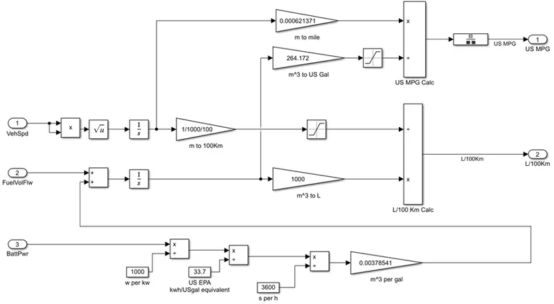
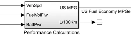
The above block is used to calculate the fuel economy in miles/gallon i.e the total amount of fuel consumed by the vehicle. Since this is an HEV, there are two sources of power involved, one is Gasoline fuel and the other is Battery Power. But, the battery power cannot be directly taken into consideration, therefore it is converted into equivalent fuel quantity.

Distance is being calculated by integrating the Vehicle Speed and is then converted into miles.

Total Fuel flow is obtained (in cubic meters) as the integration of the sum of Gasoline consumed and Equivalent fuel consumption in the case of battery. Again, the fuel flow is converted into US Gallons and with the help of a product block, the Fuel Economy in miles/US Gallon is calculated finally.

The factors considered to model the fuel flow are:

1. Vehicle Speed
2. Fuel Volume flow
3. Battery Power

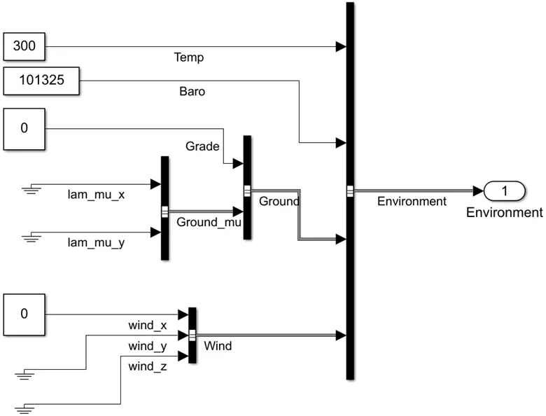
3. Observe the effects of grade & wind velocity by changing the parameters from the environment block in the HEV Reference Application (run in WOT cycle)

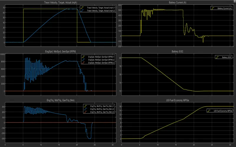
• Without any change in environmental conditions:

Output (without change in environmental conditions):

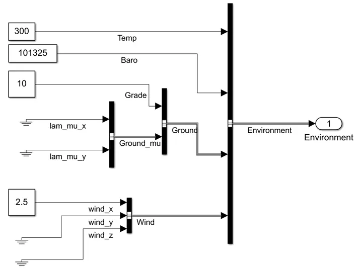
With the change in environmental conditions (Grade: 10 & Wind velocity: 2.5 m/s):

Output (with the change in environmental conditions):

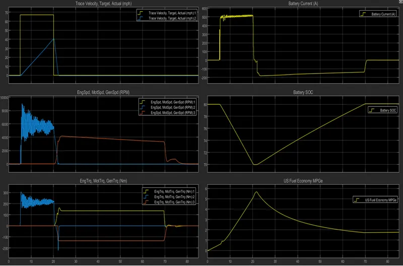
Observations:

1^st Graph: Trace Velocity (Target Vs Actual)

The yellow line indicates the target vehicle speed whereas the blue line indicates the actual speed of the vehicle. It can be observed that from 0 to 5s the vehicle was at rest, from 5 to 20s the vehicle accelerated, and then after 20s deceleration starts and finally the vehicle comes to rest.

2^nd Graph: Engine, Motor & Generator Speed (rpm)

AT the start, the battery is fully charged, therefore only the motor is in operation (indicated by blue curve). Also, it can be observed that the motor speed is high at the start to help overcome the grade & wind velocity. The engine speed (indicated by yellow curve) & generator speed (indicated by orange curve) follow the same curve and are overlapped. It can be observed that in the beginning there was no need for the engine but when the Battery SOC fell below 70% the engine started to operate to maintain the speed. Also the generator starts charging the battery at the same time to level the SOC.

3^rd Graph: Engine, Motor & Generator Torque (Nm)

It is observed that the motor torque (indicated by blue curve) is maximum at the start to help achieve maximum speed, once the objective is met i.e. constant speed is achieved, the torque requirement is decreased. It can be seen that after deceleration, for some time, the torque becomes negative indicating no torque requirement to operate and finally becomes zero i.e. the vehicle no more requires the motor to run, the engine comes into the picture and is responsible for maintaining the speed of the vehicle as can be observed that when SOC falls below 70% engine torque (indicated by yellow curve) comes into play. Also, the generator torque (indicated by the orange curve) being negative indicates the charging state.

4^th Graph: Battery Current (A)

The battery current is required only when the motor is in operation(during acceleration & running). It can be seen from the curve that initially the current demand is high when the motor was used to accelerate & run the vehicle after deceleration started the engine takeover and generator action started negative current flow (indicating charging state) started and finally, no current was withdrawn from the battery

5^th Graph: Battery SOC

The State of Charge of a battery for an EV is of utmost importance. It is analogous to a fuel gauge in the case of IC Engine vehicles. It provides data to the driver of how much longer the battery can perform before it needs to be charged. From the graph, it can be observed that when the SOC falls below 70%, it goes back into charging mode with the help of a generator driven by the engine, and the SOC is restored back.

6^th Graph: US Fuel Economy MPGe

The graph gives us the equivalent fuel required to run the vehicle in miles per gallon.

4. Comparison of simulated results of hybrid & electric powertrain.

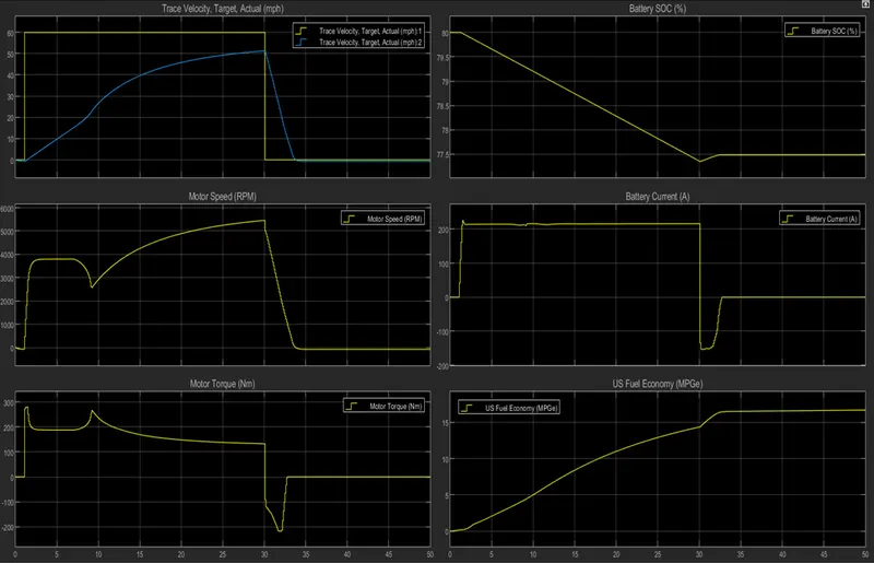
Keeping the same environmental conditions i.e. Grade: 10 & Wind velocity: 2.5 m/s the following are the outputs for pure EV & HEV.

• Pure EV output:

• HEV output:

Observations (comparison of pure EV with HEV):

1. Pure EV can attain a higher speed than HEVs as can be observed from the graphs. The Pure EV has attained a maximum speed of over 50 mph whereas the HEV could only cross 40 mph.
2. In the case of EV, it can be observed that there’s less fluctuation in motor speed compared to HEV. Also, there’s minimal fluctuation in the motor torque in the case of EV compared to HEV. However, the motor speed is more in the case of HEV when compared to EV.
3. In pure EV case it can be observed that there’s minimal fluctuation in Battery Current whereas in the case of HEV, there’s a good amount of fluctuation in the Battery current.
4. In the case of EV, it can be seen that the Battery SOC does not fall below 77% whereas in the case of HEV it fell to 70%. Also in EV a little bit of battery charging can be observed during deceleration mode

CONCLUSION:

It can be concluded that Mapped models although are fast to work with but do not produce accurate results like dynamic models which work upon real-time inputs rather than pre-defined inputs. Also, it can be concluded that environmental parameters do play an important role in the operation of a vehicle.