Week-3 Challenge: ADVISOR Tool

AIM:

To get acquainted with the features and functions of the ADVISOR (ADvanced VehIcle SimulatOR) tool.

OBJECTIVE:

1. To launch the EV_defaults_in file in the ADVISOR tool and change the cargo mass to 500 kg, with all other parameters set to their default values simulate & observe whether the vehicle can be driven for 45 km in the FTP cycle.
2. For the same EV_defaults_in file, with the cargo mass changed to 500 kg and all other parameters set to their default values, change the battery capacity & simulate the vehicle in the FTP cycle.
3. To perform gradeability test on the PRIUS_Jpn_defaults_in file and compare the results in a tabular format.

ADVISOR (ADvanced VehIcle SimulatOR) tool:

What is ADVISOR?

ADVISOR, NREL’s ADvanced VehIcle SimulatOR, is a set of model, data, and script text files for use with Matlab and Simulink. It is designed for rapid analysis of the performance and fuel economy of conventional, electric, and hybrid vehicles. ADVISOR also provides a backbone for the detailed simulation and analysis of user-defined drivetrain components, a starting point of verified vehicle data and algorithms from which to take full advantage of the modeling flexibility of Simulink and analytic power of MATLAB.

ADVISOR helps us to

• estimate the fuel economy of vehicles that have not yet been built
• learn about how conventional, hybrid or electric vehicles use (and lose) energy throughout their drivetrains
• compare relative tailpipe emissions produced on a number of cycles
• evaluate an energy management strategy for your hybrid vehicle’s fuel converter
• optimize the gear ratios in your transmission to minimize fuel use or maximize performance, etc.

The models in ADVISOR are:

• mostly empirical, relying on drivetrain component input/output relationships measured in the laboratory, and
• quasi-static, using data collected in steady-state (for example, constant torque and speed) tests and correcting them for transient effects such as the rotational inertia of drivetrain components.

Capabilities of ADVISOR tool:

ADVISOR uses basic physics and measured component performance to model existing or future vehicles. Its real power lies in the prediction of the performance of vehicles that have not yet been built. It answers the question “what if we build a car with certain characteristics?” ADVISOR usually predicts fuel use, tailpipe emissions, acceleration performance, and gradeability.

In general, the user takes two steps:

1. Define a vehicle using measured or estimated components and overall vehicle data.
2. Prescribe a speed versus time trace, along with road grade, that the vehicle must follow.

ADVISOR then puts the vehicle through its paces, making sure it meets the cycle to the best of its ability and measuring (or offering the opportunity to measure) just about every torque, speed, voltage, current, and power passed from one component to another.

ADVISOR allows us to answer questions like:

• Was the vehicle able to follow the speed trace?
• How much fuel and/or electric energy were required in the attempt?
• How does the state-of-charge of the batteries fluctuate throughout a cycle?
• What were the peak powers delivered by the drivetrain components?
• What was the distribution of torques and speeds that the piston engine delivered?
• What was the average efficiency of the transmission?

By iteratively changing the vehicle definition and/or driving cycle, we can go on to answer questions such as:

• At what road grade can the vehicle maintain 55 mph indefinitely?
• What’s the smallest engine I can put into this vehicle to accelerate from 0 to 60 mph in 12 s?
• What’s the final drive ratio that minimizes fuel use while keeping the 40 to 60 mph time below 3 s?
• What is the fuel economy sensitivity to mass, aerodynamic drag, or other vehicle or component variations?

ADVISOR’s GUI and other script files answer many of these questions automatically, while others require some custom programming on the user’s part.

Because ADVISOR is modular, its component models can be relatively easily extended and improved. For example, an electrochemical model of a battery, complete with diffusion, polarization, and thermal effects, can easily be put into a vehicle to cooperate with a motor model that uses a measured efficiency map.

Limitations of ADVISOR tool:

• Primarily for analysis, not design: ADVISOR was developed as an analysis tool, and not originally intended as a detailed design tool. Its component models are quasi-static, and cannot be used to predict phenomena with a time scale of less than a tenth of a second or so. Physical vibrations, electric field oscillations, and other dynamics cannot be captured using ADVISOR, however recent linkages with other tools such as Saber, Simplorer, and Sinda/Fluint allow a detailed study of these transients in those tools with the vehicle level impacts linked back into ADVISOR.

  As an analysis tool, ADVISOR takes the required/desired speed as an input and determines what drivetrain torques, speeds, and powers would be required to meet that vehicle speed. Because of this flow of information back through the drivetrain, from the tire to axle to gearbox and so on, ADVISOR is what is called a backward-facing vehicle simulation.

  Forward-facing vehicle simulations include a model of a driver, who senses the required speed and responds with an accelerator or brake position, to which the drivetrain responds with a torque. This type of simulation is well suited to the design of control systems, for example, down to the integrated circuit and PC card level—the implementation level.

  ADVISOR is well suited to evaluate and, by iterative evaluation, design control logic and energy management strategies. By this, we mean something like “When the engine torque output is low and the battery state of charge is high, turn off the engine.” The control logic, with which ADVISOR can work, is about what you want the vehicle to do. The detailed control system, getting into details of how you would implement this control logic in hardware, is about how to make the vehicle do what you want and is not the original intention of ADVISOR’s application.

• Power bus for electric power transfers: In electrical components’ communication with each other, ADVISOR deals in power, and not in voltage and current. Linkages to other tools, such as Saber and Simplorer let the user work with a voltage bus.

• Drive axle is single axle only: The vehicle dynamics calculations required for traction control and the wheel slip model assume that the front axle is the only drive axle. Simple steps can be taken to correct the weight transfer calculation if you wish to model a rear-drive vehicle and an example wheel file that accomplishes this is included. Modeling a four-wheel-drive vehicle requires involved Simulink reprogramming

STUDY:

I. For EV_defaults_in file, if cargo mass is 500 kg with all other default conditions, can the vehicle travel for 45 km with FTP drive cycle?

In the MATLAB window, the path was changed to the folder where the ADVISOR tool was stored. Then in the command window, the "advisor" command was run to start the ADVISOR tool. Once the start window appeared "Metric" system of units was selected and then the "Start" button was used to launch the tool.

After the launch, from under the "Load file" dropdown, the "EV_defaults_in" was selected. Once the file got loaded the Cargo Mass was changed to 500kg as specified in the question.

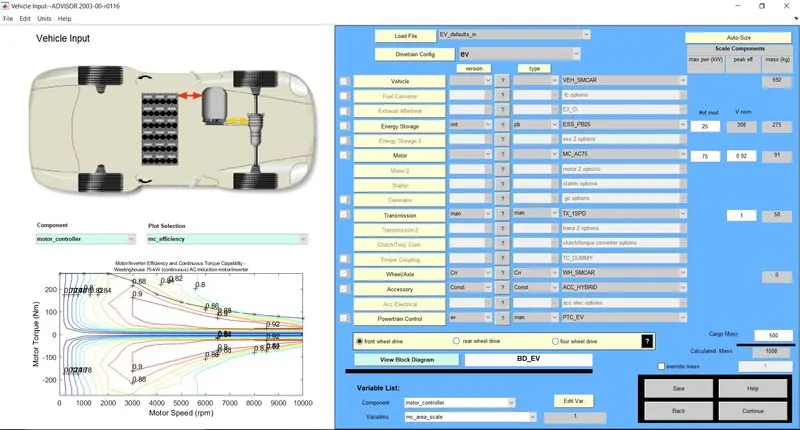
Then the "Continue" tab was clicked upon, following which the tool navigated to another page where the Drive Cycle was changed to FTP via the dropdown.

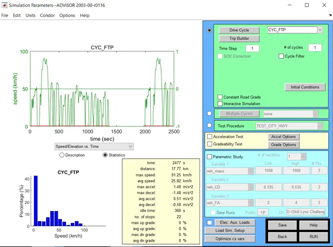
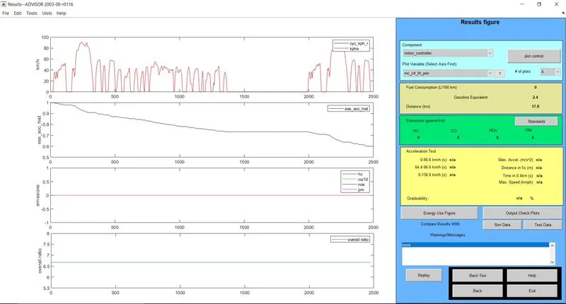
Now, the simulation file was executed initially for only 1 drive cycle and it was found that the vehicle drove to a distance of 17.8 km with 40% battery consumption as shown below:

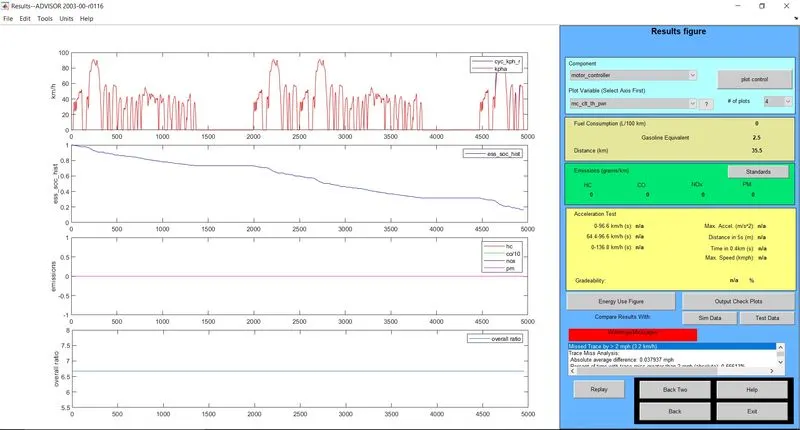
Again, the simulation was executed now with 2 drive cycles and it was observed that the vehicle drove to a distance of 35.5 km with approximately 83% battery consumption.

Since, our objective was to cover a distance of 45 km, this time we executed the simulation with 3 drive cycles and it was observed that the vehicle drove to a distance of 41.4 km after which the charge was exhausted.

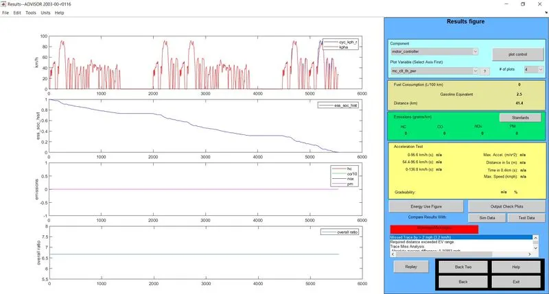
Observation: In a single charge with the given battery module, the vehicle could not drive up to 45 km in the FTP Drive cycle.

2. For Study 1, try changing the battery capacity & repeat the simulation.

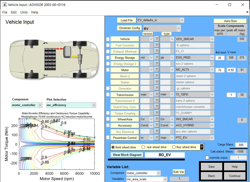
Initially, the number of modules was 25 with a nominal voltage of 308V as shown below:

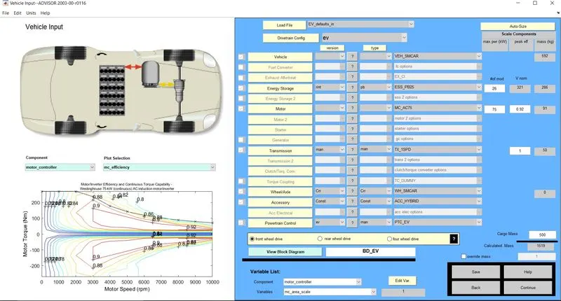
Now, as asked in the question, for the first instance the number of battery modules was increased by 1, i.e. Total no. of modules = 26 & Nominal Battery Voltage = 321 V as shown below:

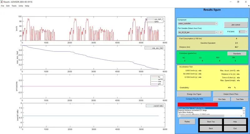
Now, the model was simulated for 3 FTP Drive Cycle and it was found that the vehicle could travel only up to 42.7 km as shown below:

Then, again the number of modules was increased by 1 for the second time, i.e. Total no. of modules = 27 & Nominal Battery Voltage = 333 V as shown below:

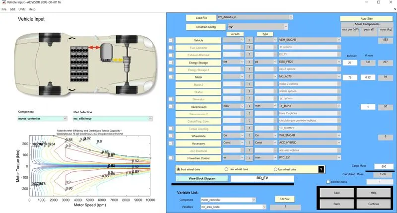
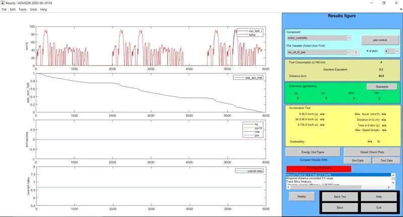
Again, the updated model was simulated for 3 FTP Drive Cycle and it was found that the vehicle could travel up to 44.8 km (near the 45km mark but not 45km exactly) as shown below:

Again, the number of modules was increased by 1 for the third time, i.e. Total no. of modules = 28 & Nominal Battery Voltage = 345 V as shown below:

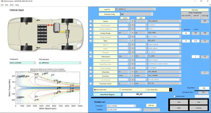
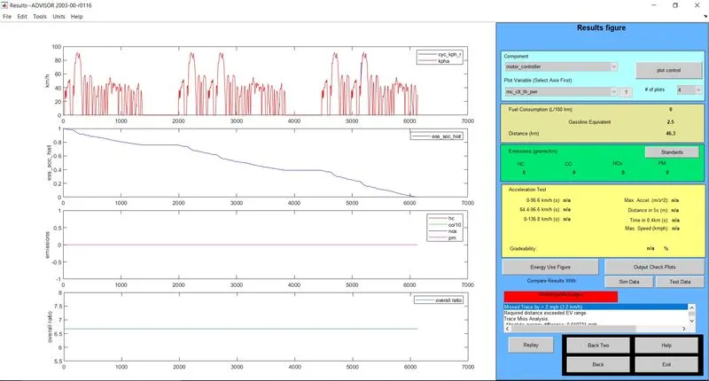
Once again, the updated model was simulated for 3 FTP Drive Cycle and it was found that this time with a 28 module battery having a nominal voltage of 345V the vehicle could travel up to 46.3 km (well beyond 45km) as shown below:

Observation: An increase in battery capacity i.e. addition of 3 modules helped achieve the desired range of 45 km on a single charge on an FTP Drive Cycle.

3. Gradeability test on the PRIUS_Jpn_defaults_in file and comparison of results:

Gradeability of a vehicle is its ability to climb slopes. Gradeability is measured either in degrees or percentages. A 45 degrees gradient is equivalent to 100 percent. Gradability is dependent on engine power, drivetrain type, gear ratio, weight, weight distribution, car's center of gravity, and traction.

The time duration was kept fixed at 10 seconds, and the speed of the vehicle was varied in multiples of 10 i.e. 10mph, 20mph, 30mph, 40mph, 50mph & 60mph, and then the PRIUS_Jpn_defaults_in file was simulated for each value of speed and the Gradeability percentage was observed which is shown below in screenshots:

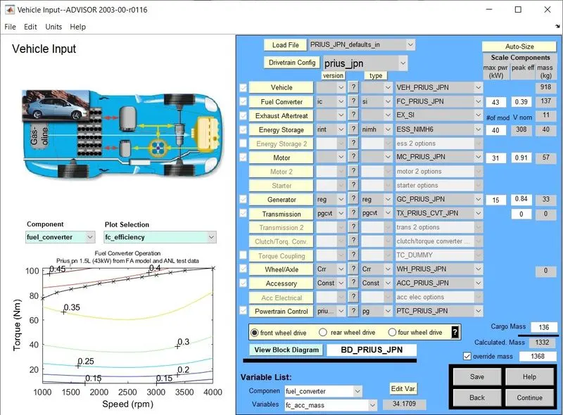
The base file of the PRIUS_Jpn_defaults_in:

All parameters in this particular sheet are set to default.

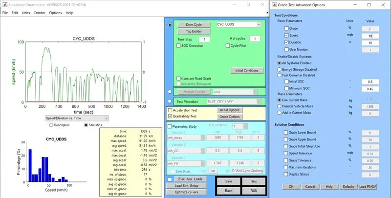
INPUT SPEED & OUTPUT GRADEABILITY of the said vehicle can be observed as under:

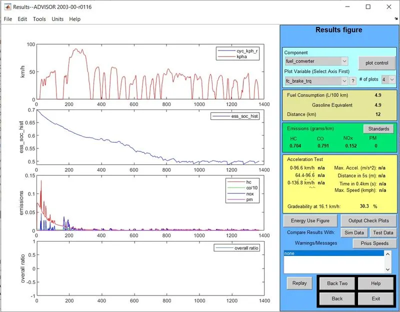
i. For 10mph i.e. 16.1 km/hr, Gradeability was observed to be 30.3%

Input:- Speed setting: 10mph

Output:- Gradeability: 30.3%

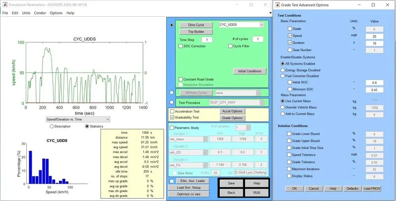
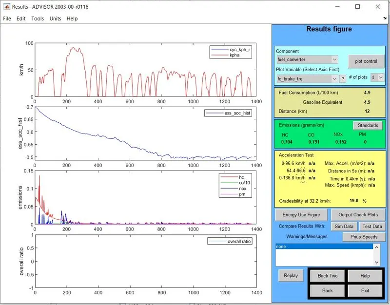
ii. For 20mph i.e. 32.2 km/hr, Gradeability was observed to be 19.8%

Input:- Speed setting: 20mph

Output:- Gradeability: 19.8%

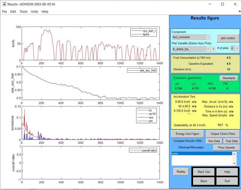
iii. For 30mph i.e. 48.3 km/hr, Gradeability was observed to be 14.7%

Input:- Speed setting: 30mph

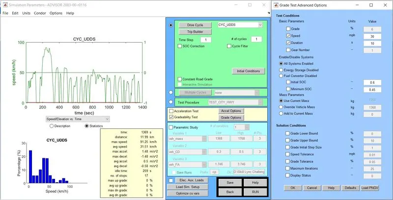
Output:- Gradeability: 14.7%

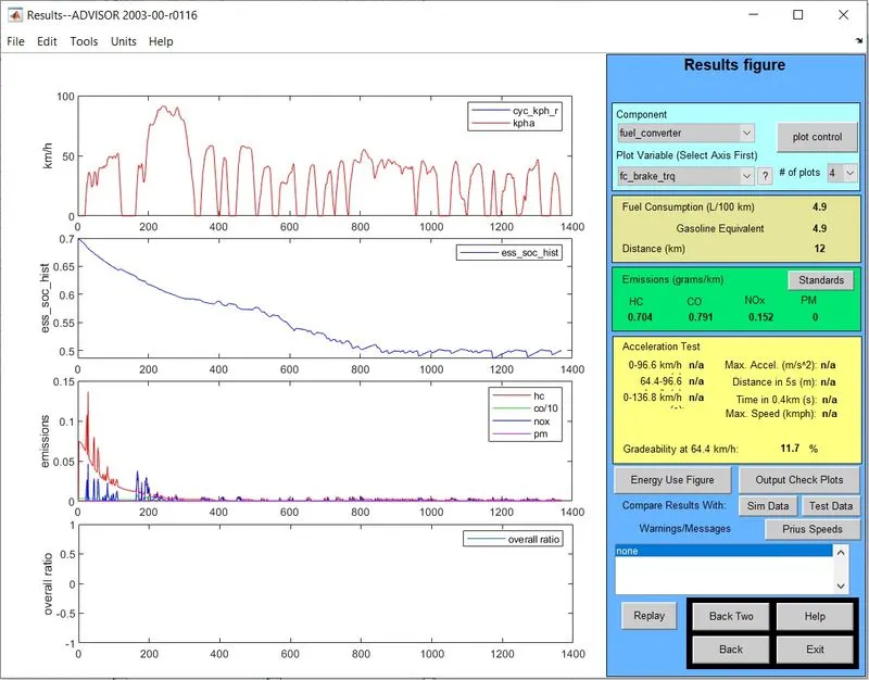
iv. For 40mph i.e. 64.4 km/hr, Gradeability was observed to be 11.7%

Input:- Speed setting: 40mph

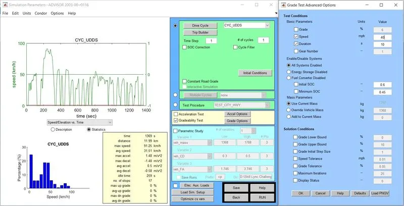
Output:- Gradeability: 11.7%

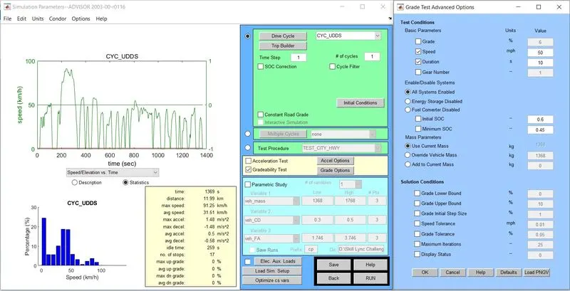
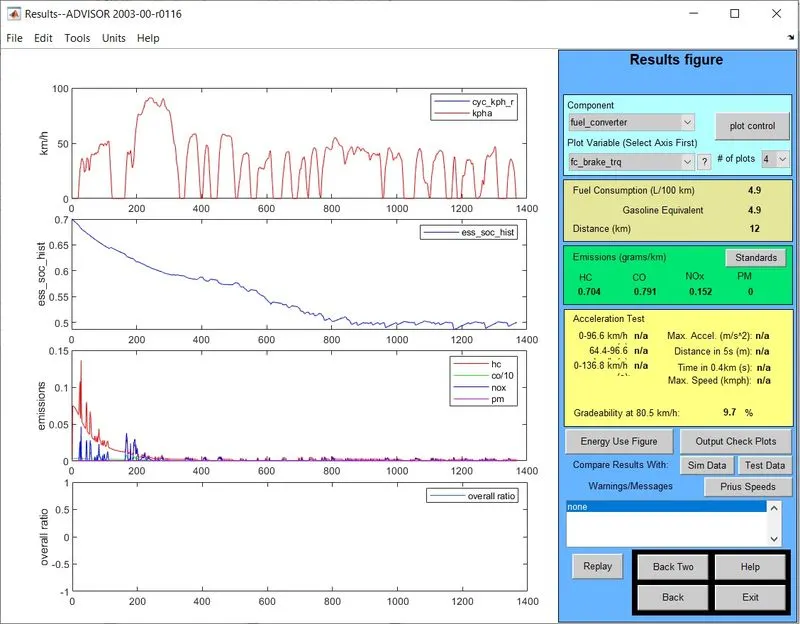
v. For 50mph i.e. 80.5 km/hr, Gradeability was observed to be 9.7%

Input:- Speed setting: 50mph

Output:- Gradeability: 9.7%

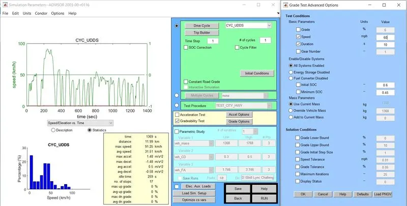
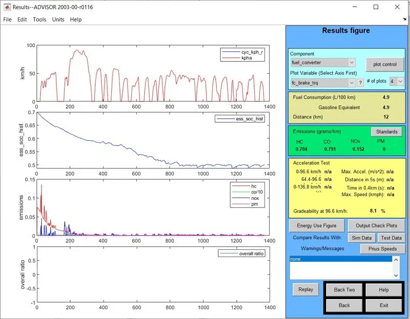
vi. For 60mph i.e. 96.6 km/hr, Gradeability was observed to be 8.1%

Input:- Speed setting: 60mph

Output:- Gradeability: 8.1%

For 10 second duration, variation in Gradeability w.r.t change in Speed is shown below in the tabular format:

Sl.No.	Time (sec)	Speed (mph)	Speed (km/h)	Gradeability (%)
1	10	10	16.1	30.3
2	10	20	32.2	19.8
3	10	30	48.3	14.7
4	10	40	64.4	11.7
5	10	50	80.5	9.7
6	10	60	96.6	8.1

The above table has been uploaded as an Excel sheet. The data was imported in MATLAB from the excel sheet taking only the Speed(km/h) & Gradeability data as column vectors which were then loaded into the Base Workspace with the variable names as "Speedkmph" & "Gradeability". The following code was written to obtain a plot of the Gradeability Vs Speed curve (m-file has been uploaded along with the Assignment):

% Code for Gradeability Vs Speed plot
plot(Speedkmph,Gradeability);
xlabel('Speed (kmph)');
ylabel('Gradeability (%)');
title('Plot of Gradeability Vs Speed');

The plot of Gradeability Vs Speed with the above code:

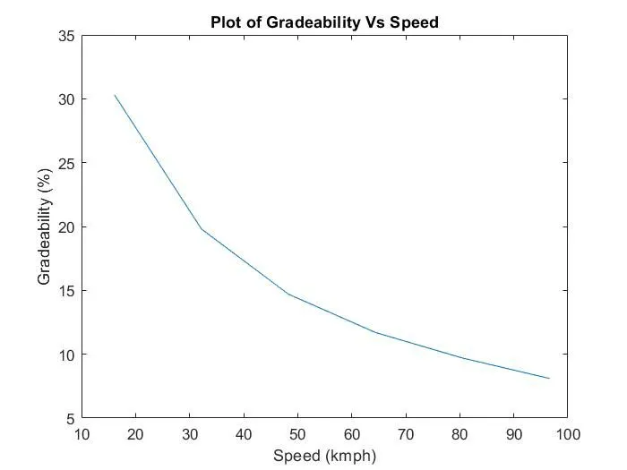
Observation: From the above plot it can be observed that Gradeability of a vehicle decreases exponentially with increase in speed.

CONCLUSION:

In an Electric Vehicle the SOC matters a lot, also the battery modules have an important role to play in the driving range of the vehicle. As can be observed from the Question 1 & 2 that a slight increase in the battery module incresed the range of the vehicle. Also from the Question 3 we can observe that the Gradeability of a vehicle decreases exponentially with the increase in speed of the vehicle.

REFERENCE:

i. ADVISOR Tool Details - http://adv-vehicle-sim.sourceforge.net/

ii. ADVISOR Tool Download - https://sourceforge.net/projects/adv-vehicle-sim/files/latest/download

iii. ADVISOR Tool DIscussion Forum - https://groups.google.com/g/adv-vehicle-sim