WOT Condition Part-2

1. What is the difference between the mapped and dynamic models of engine, motor, and generator? How can you change the model type?

The major difference between the mapped and dynamic models are explained below in terms of an engine.

Mapped type - (CiMappedEngine, SiMappedEngine)

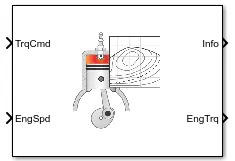
The model uses a set of steady-state lookup tables to characterize engine performance. The tables provide overall engine characteristics, including actual torque, fuel flow rate, BSFC, and engine-out exhaust emissions. We use this block if we have engine data from a dynamometer or a design tool like GT-POWER, and also for quasi-steady-state engine simulations.

Dynamic type - (CiEngine, SiEngine)


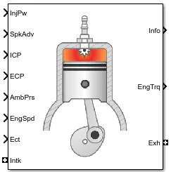
The model decomposes the engine behavior into engine characteristics that are separated into lower-level components. By combining components in this way, the models capture the dynamic effects. We use it when we need a more detailed dynamic model and have component-level data and also to analyze the impact of individual engine components on the overall performance.

The same goes for the mapped and dynamic models of a motor and generator.

Further to summarize the differences -

1. If we need a more detailed and accurate dynamic analysis, we need to use the dynamic variant and if we need to have a faster execution of the model, we need to use the mapped variant.
2. The mapped variant is used for a system-level simulation where we do not know the detailed parameters of the engine, motor, or generator. Whereas, a dynamic variant is used for a component-level simulation where we know all the detailed parameters of the engine, motor, or generator.
3. The mapped variant uses a look-up table to calculate the values and obtain results whereas the dynamic variant uses the input data we provide for the calculations.

Now in the example model of the powertrain blockset, we have the option of using both the mapped and dynamic models for obtaining the results as per requirement. The image below shows us the mapped model selected as default.

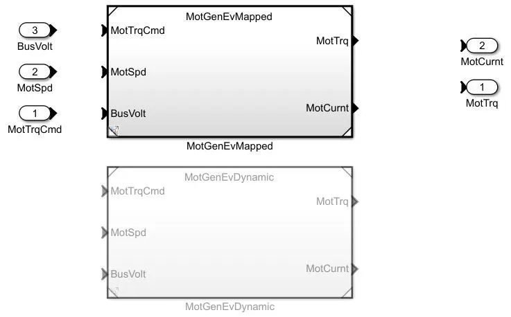
To change the model from mapped to dynamic, we need to follow the below-mentioned steps

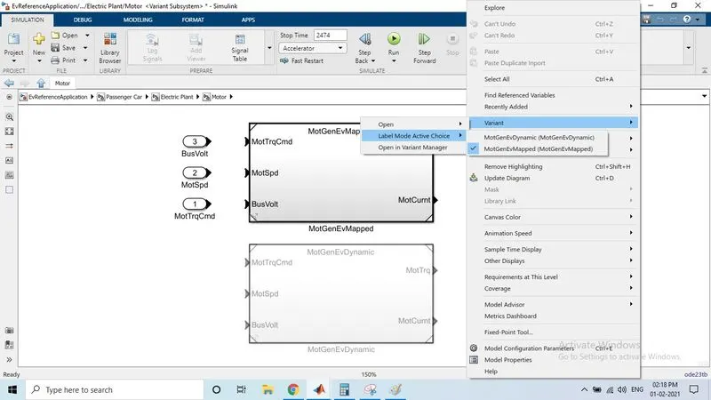
Right-click on the blank space --> Select variant --> Select label mode active choice --> Select 'MotoGenEvDynamic'

The below image shows the steps required to be taken.

2. How does the model calculate miles per gallon? Which factors are considered to model fuel flow?

The below image is from the hybrid vehicle multimode reference application from the powertrain blockset example. It shows us the method to calculate miles per gallon.

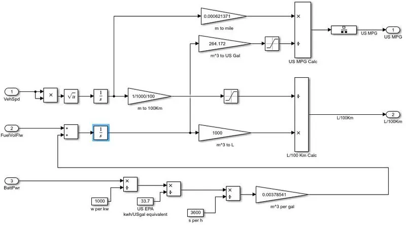
The procedure followed using the Simulink blocks as shown is explained below -

1. The vehicle speed is multiplied by itself using the product block and then the square root of the value is taken using the sqrt block . This procedure is to make sure that the values are not negative before integration.
2. The next step is to integrate the vehicle speed to get the distance covered by the vehicle i.e., converting the value from m/s to m. The integration is done using the integrator block.
3. Now, we need to convert meters to miles. We know that 1m = 0.000621371 miles. Hence we use the gain block to multiply our value with the conversion unit and obtain the result in miles.
4. The next step is to consider the fuel flow and battery power and then convert them into gallons. The battery power value which is in Watts (W) should be converted into m^3/gal. We can observe that the value will be divided by the value '1000' to be converted from W to kW and 33.7 to be converted into 'US EPA or kWh/USignal equivalent' and also by 3600 to be converted from seconds to an hour. The obtained value will now be converted into m^3/gallon using the gain block and multiplying the value with the conversion unit of 0.00378541.
5. The battery power which is converted to m^3/gallon is added with the value of fuel flow and then will be integrated using the 'integrate' block to obtain the value in m^3 units from m^3/gallon.
6. Now the value of the sum of fuel flow and battery power in the m^3 units will be converted into US gal using the gain block and multiplying the same with the conversion value of 264.172.
7. This value will be limited to its upper and lower limits using the 'saturation' block. The upper limit being infinity and the lower limit being '1e-3'.
8. Now the distance covered by the vehicle which is in miles and the sum of fuel flow and battery power which is in US gal will be divided to obtain the result as required by us. A rate transition block is used here to handle the data transfer smoothly.

This is how the model calculates miles per gallon.

For the model fuel flow, the factors considered are -

1. Vehicle speed through which we find out the distance covered
2. Fuel flow, the volume of fuel used by the vehicle to cover that distance
3. Battery power that is consumed by the vehicle to cover that distance

The fuel flow is measured in L/100km.

3. Run the HEV ReferenceApplication with WOT drive cycle. Change the grade and wind velocity in the environment block. Comment on the results.

We are exploring the hybrid electric vehicle multimode reference application as an example in the powertrain blockset available in Simulink. The main model is shown below.

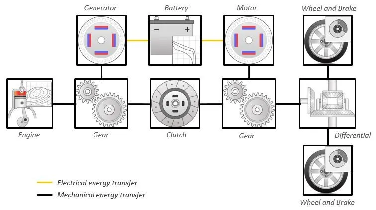
It is an example of a backward flow arrangement. By default, the drive cycle that is selected would be 'FTP75'. There are many subsystems included in this model, the environment subsystem, the longitudinal driver, the controllers, the passenger car subsystem, and the visualization subsystem which will consist of the scope and results.

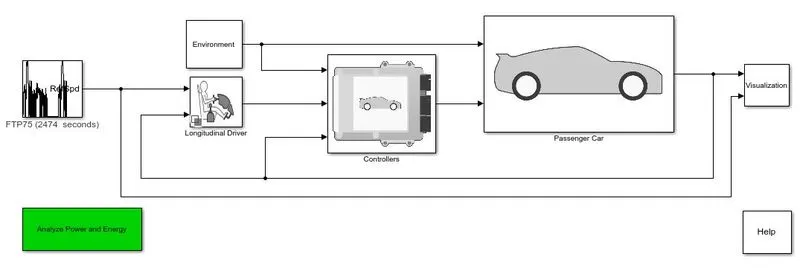
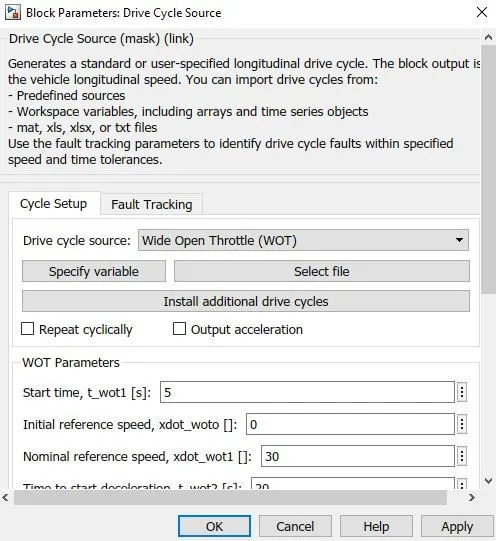
Now as per the requirements, the drive cycle source must be changed from 'FTP75' to 'Wide Open Throttle (WOT)' as shown in the below image.

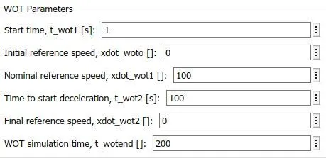
The WOT parameters are changed as per my assumptions and are shown below -

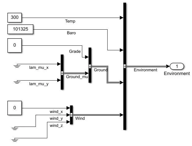
Once we select the WOT condition and decide on the parameters, we have to change the grade and wind velocity values. We can do that by going into the environment subsystem.

The below images shows the environment subsystem and we have changed the grade value from 0 to 6%, and the wind velocity from 0 to 10 mph.

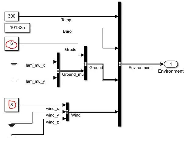
With the top speed of the cycle being 100 m/s, cycle time being 200 sec, and time to start deceleration being 100 sec, grade being 6% and wind velocity being 8m/s, we obtain the below plots as shown.

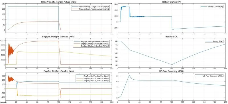
The above figure shows the results for the simulation and there are a total of six plots in them.

Plot 1 - shows the velocity of the vehicle concerning driving cycle data with the time scale on the x-axis. The vehicle reaches a maximum of 80 m/s as there are other forces acting on it.

Plot 2 - shows the changes in the speed of the engine, motor, and generator in RPM throughout the time scale in the x-axis.

Plot 3 - shows torque characteristics and its changes of the engine, motor, and generator in Nm throughout the drive cycle.

Plot 4 - shows the battery current values (A) and their changes for various acceleration inputs as per the drive cycle. The peak current discharge is at 500 Amps and the peak current charge is at -200 Amps.

Plot 5 - shows the battery state of charge SOC(%) and its changes corresponding to the driving inputs. The battery SOC dropped from 80% to 50% in 100 seconds at the provided conditions.

Plot 6 - shows the fuel economy as a mile per gallon for the corresponding input driving conditions.

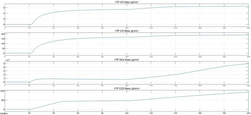
The above plot shows the TP emission scope obtained by the data through the HEV.

4. Keeping all other parameters the same, compare the simulated results of hybrid and pure electric powertrains.

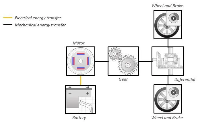
The above image shows us the EV reference model. Now we run this model similar to the HEV reference model keeping all the parameters the same. The parameters are listed below.

1. The top speed of the cycle = 100 m/s

2. Cycle time = 200 sec

3. Time to start deceleration = 100 sec

4. Grade = 6%

5. Wind velocity = 8m/s

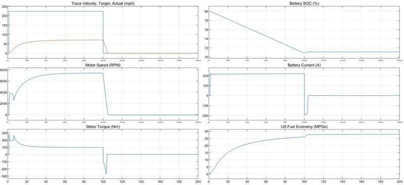
The above results comprise of 6 plots and each of them is explained below.

Plot 1 - shows the velocity of the vehicle with respect to the drive cycle data with the time scale on the x-axis. The top speed achieved is approximately around 75 m/s as there are other forces acting on it.

Plot 2 - shows the changes in the speed of the motor in RPM throughout the drive cycle.

Plot 3 - shows the torque characteristics and its changes of the motor in Nm throughout the drive cycle.

Plot 4 - shows the battery state of charge SOC (%) and its changes corresponding to the driving inputs. The battery drops from 80% to 71% in 100 sec for the given driving conditions.

Plot 5 - shows the battery current and its changes for various acceleration inputs as per the drive cycle. The maximum current discharged is 200 Amps and the maximum current charged is -200 Amps.

Plot 6 - shows the equivalent fuel economy as a mile per gallon for the corresponding input driving conditions.

Comparison between a pure electric and a hybrid electric vehicle with the same load conditions -

1. The EV when compared with an HEV with the same environmental and drive cycle conditions result in less top speed achievement.
2. The electric vehicle produces high motor speed and torque when compared with an HEV, but an HEV when combines the torque of both motor and engine is higher than an EV torque. This is why the HEV is faster compared to the EV in the above results.
3. The discharging capacity and the rate of charging is higher in the pure electric vehicle when compared with the hybrid electric vehicle.
4. The efficiency of the electric vehicle is higher than the hybrid electric vehicle.
5. The electric vehicle produces 0 emissions whereas hybrid electric vehicles produce waste gas emissions.