Week 4.2: Project - Transient simulation of flow over a throttle body

AIM:

Transient state simulation for flow over a throttle body.

Theory:

In steady state we consider the properties are not changing with time but in case of Transient flow the properties are changing with time.

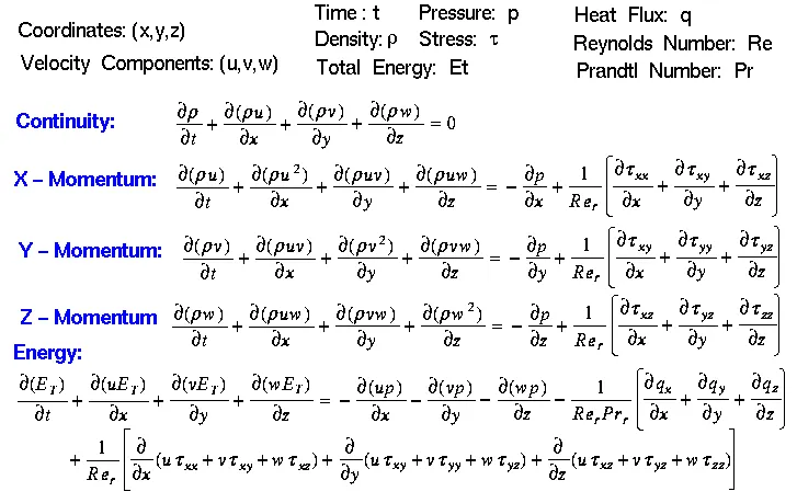
N-s Equation:

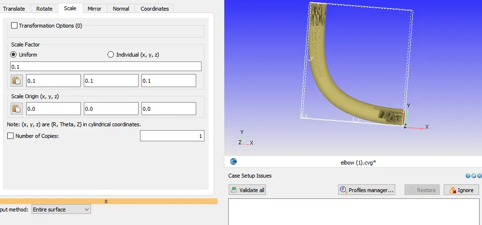
Scale :

Scale the the model to decreases mash count by 0.1.

Run Parameters:

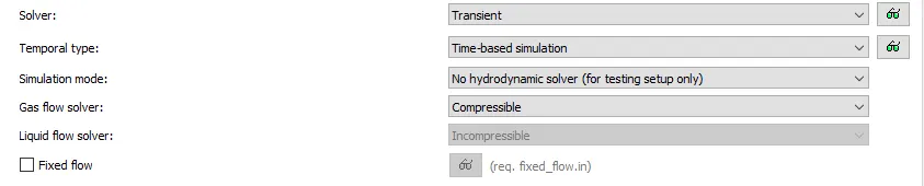
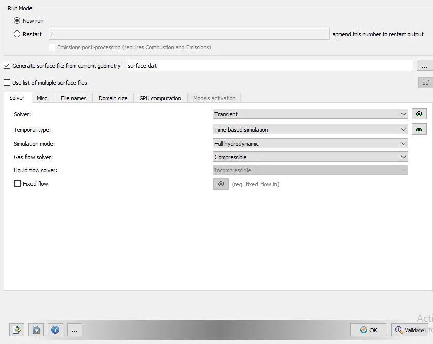
Transient solver used so the simulation is Time-based simulation. Simulation model is No hydrodynamic to analyze variable mash near the throttle valves.

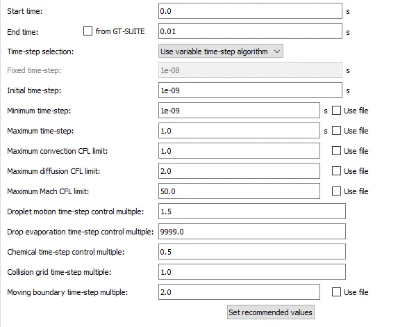
Run the simulation for 0.01 sec

Use Variable time step algorithm to control the calculation time, As it is variable mash simulation if CFL No>1 the simulation get un stable so it use variable time step size as per the required.

Boundary:

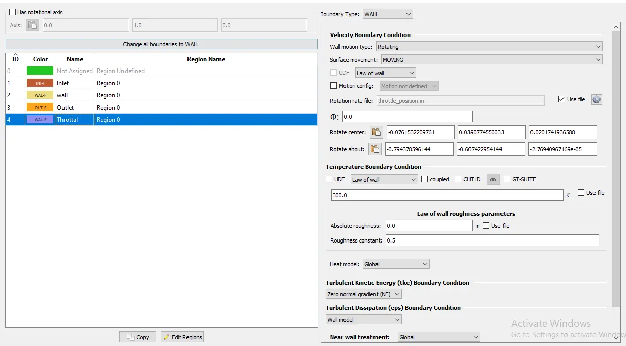
Here the throttle is rotating so the throttle is boundary is moving type.

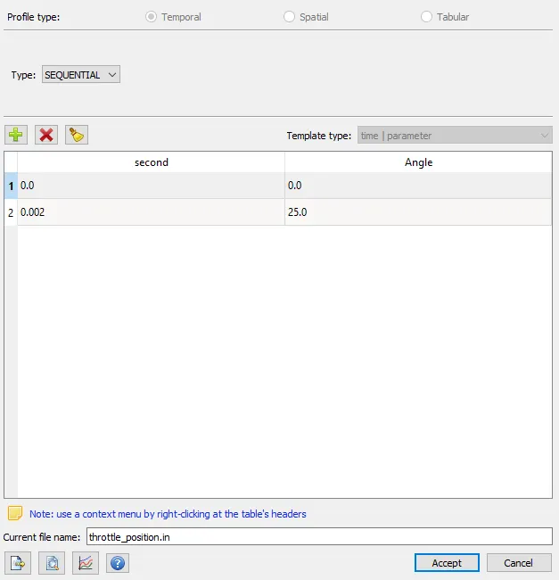
For rotation rate create throttle position file named as " theottle_position.in" . he we save location as per time at 0 sec at 0 Deg, at 0.002 sec rotate to 25 Deg.

Here the throttle rotate about the lever so the rotate center is the lever center and throttle rotate about the normal though the center.

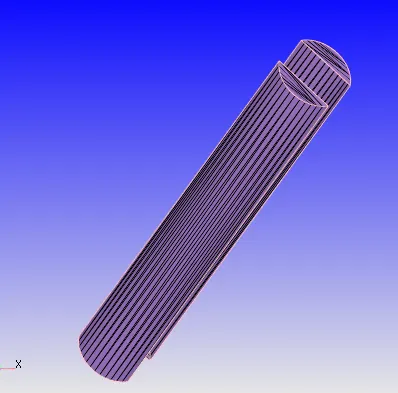
Base Grid:

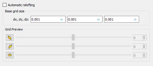
Base Grid is 0.001.

Output File:

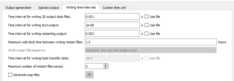
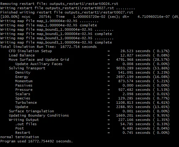
Writing output file every 0.001s, text output of the file is 1e-06s, time interval writing reset file is 0.002.

Run the No Hydrodynamic simulation:

Run the No hydrodynamic simulation to observe the setup and mash generation is correct or not.

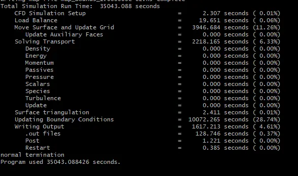
Post processing of the No Hydrodynamic simulation:

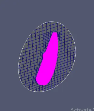
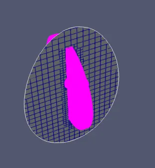
We can observe the mash is changing with time and throttle is rotating about lever.

Full Hydrodynamic simulation:

Post Processing:

Velocity:

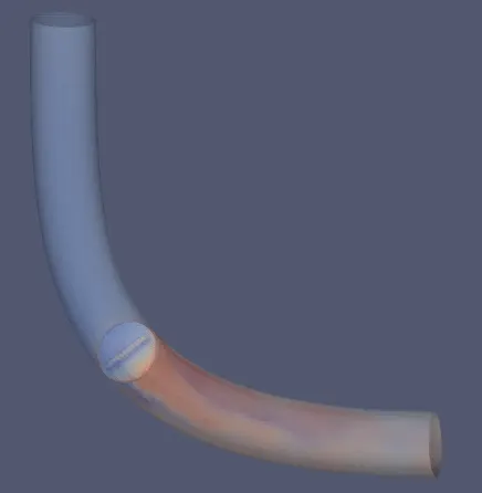
If We observe the above image and observe after throttling process the velocity of the fluid increase. these process can be understand by following images.

In pervious observation we understand aria of fluid flow decreases so the velocity increases. Here the throttle rotate to some angle so the throttle act as Nozzle. so the velocity increases is more, when the throttle rotates.

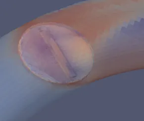
If we observe above image. Velocity near the throttle valve is Zero in the first image it is due to higher drag force on the throttle valve. In Second image there is some velocity. The first image in the direction of rotation side and second image in opposite side. so there resistive force opposite to the direction of rotation.

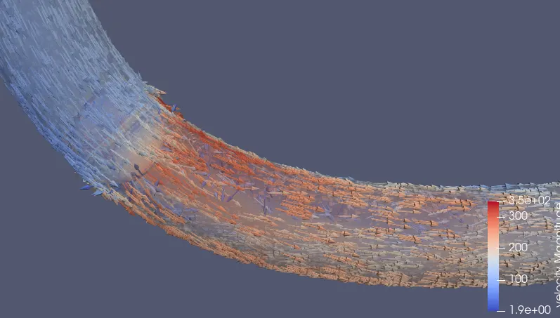
Here it showing Velocity vectors.

We can see here some fluid particles are circulating after throttle valve. it is due to wake region after throttle valve.

Pressure:

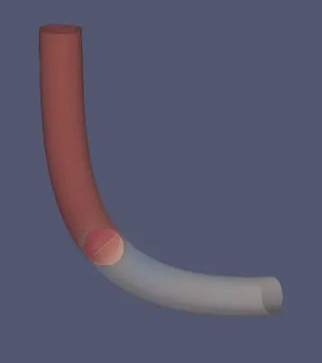
In previous Observation we observe throttling process is a expansion process. Here we can observe if we close the valve, there is more pressure loss. This is due ' After throttling velocity increases so dynamic pressure increases but static pressure decreases.

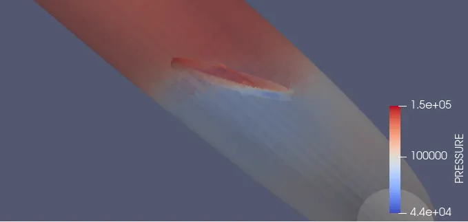
Here we can observe there is pressure force on the throttle valve opposite to direction of rotation.

Average value at Inlet And outlet:

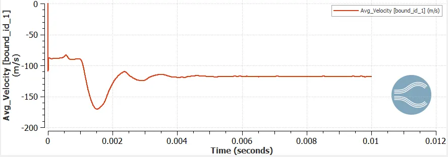
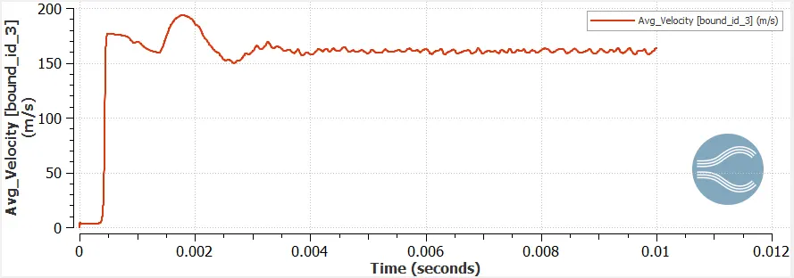
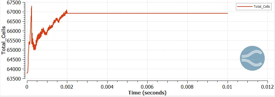
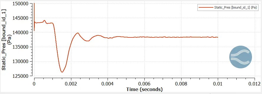
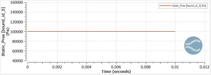
In above all the plot We can observe after 2 sec the variables are start stable. this is due the valve opining time.

In inlet the velocity is -ve because the direction of flow opposite to the normal of the surface normal and after the valve fully open the average outlet velocity increases.

In the cell count plot we can see as valve rotation increases the cell count increases.

The static pressure at out let is constant but at inlet changing .Its due when the valve open there is restriction in fluid flow.