Week 4.2: Project - Transient simulation of flow over a throttle body

Aim: The aim of the project is to simulate the flow through a throttle body using transient simulation. The objective is to understand the development of the flow with the aid of different plots.

Theory:

The throttle valve arrangement which is the subject of this analysis is frequently used in automobiles to regulate the air-fuel mixture in the combustion engine. Butterfly valves are the most commonly used valves. In this analysis, we would be examining the results under the assumption of transient conditions.

Throttling is an Isenthalpic process.

Case Setup:-

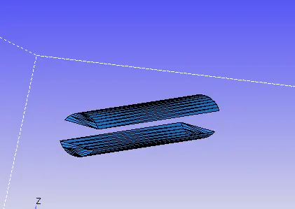
1. Geometry Creation:- The geometry that was used for the analysis is shown below. An STL file was imported into CONVERGE. It comprised a number of open edges that were cleaned using a Patch command.

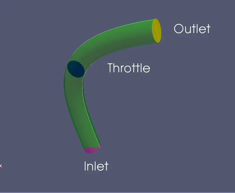
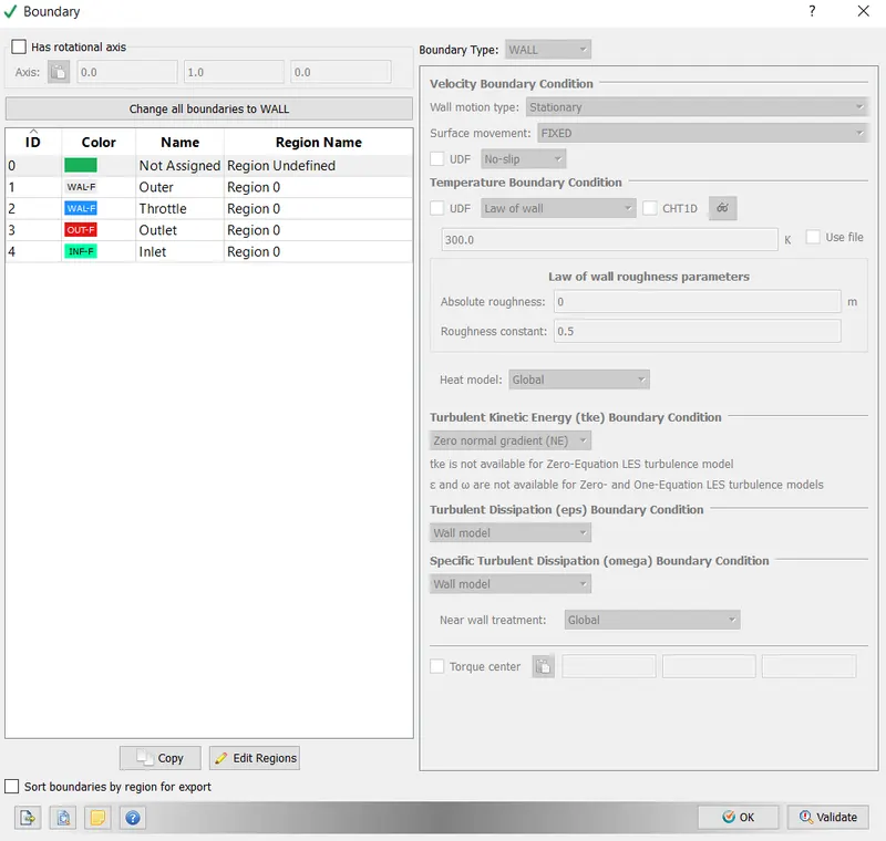
1. Creation of Boundaries: In the geometry which is created above, boundaries such as inlet, outlet, outer body, and throttle.

1. Checking Orientation of Normals: The orientation of Normals was checked to ensure all the normals are pointing inwards. This was done using the Normal Toggle
2. Finally, a Diagnosis check was run to ensure no errors in the geometry.

B Case Setup

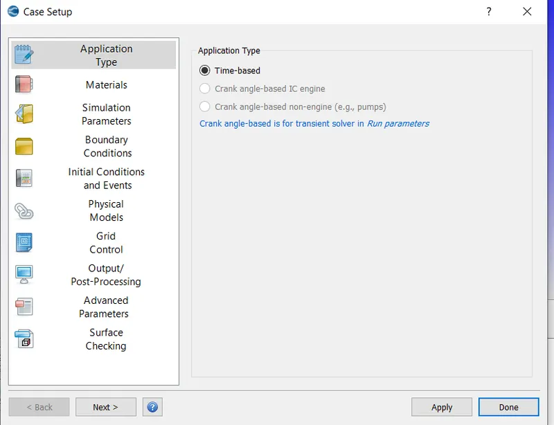
1. Application Type:- This was set to Time-based

2. Materials:- This was set to Air

1. i) Gas Simulation: Default properties were retained
2. ii) Global Transport Parameters:- Default properties retained
3. Simulation Parameters

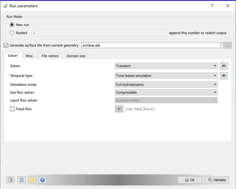
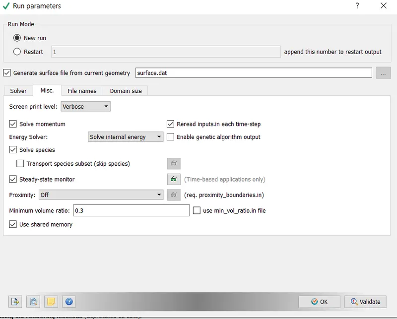
- Run Parameters:- Steady state solver was used. The simulation mode was set to Full Hydrodynamic. The gas flow solver is set to Compressible

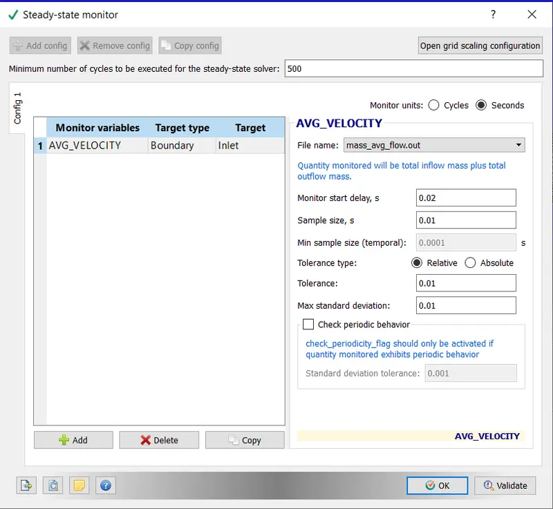
- Steady State Monitor:- Minimum no of cycles to be executed for Steady-state solver -500

Monitor Start Delay, Seconds:- 0.02

Sample size seconds:- 0.01

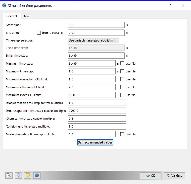
- Simulation Time Parameters:- The parameters were set as displayed below. Max CFL limit set to 1.0

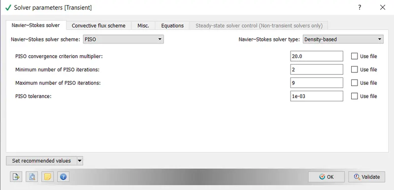
- Solver Parameters:- A Pressure based PISO solver was used, Maximum Convection CFL limit was set to 0.5.

4. Boundary

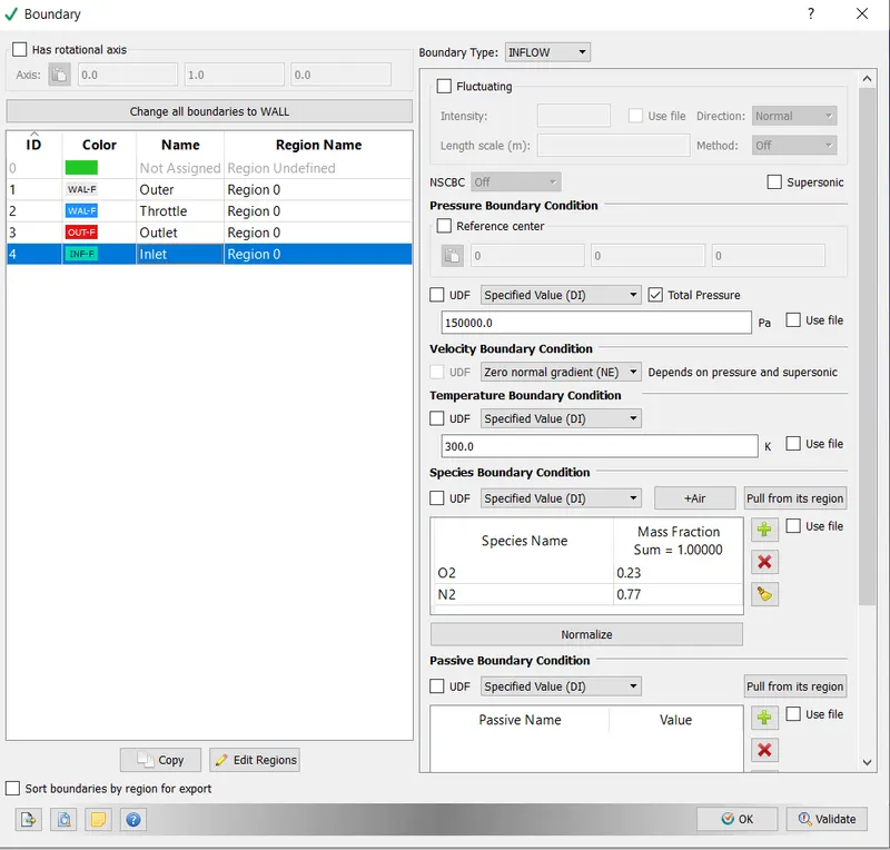
- Inlet:- Boundary flow - Inflow

Inlet Pressure- 150000 Pa

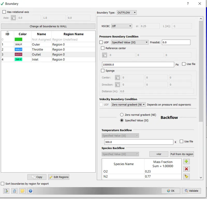
- Outlet- Boundary - Outflow

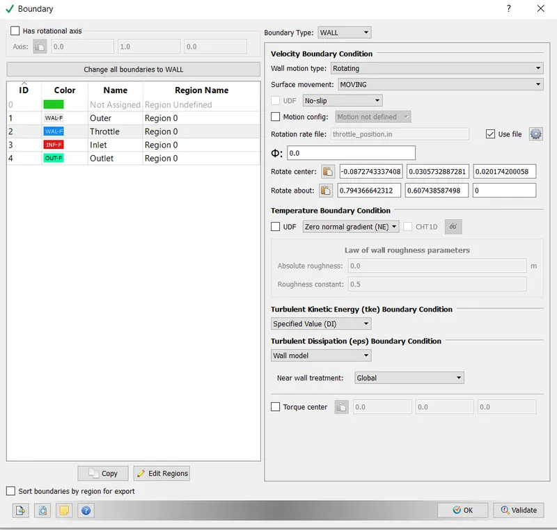
- Throttle:- Wall motion was set to Rotating, Surface Movement:- Moving.

The center and axis of rotation were determined by using the Measure command and Direction Arc Normal. Three points need to be specified to compute the rod center.

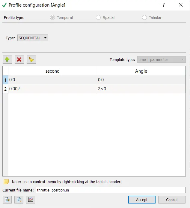
Also, the angle of throttle movement was set using the rotation rate file, from 0 to 2 milliseconds the valve would turn between 0 and 25 degrees.

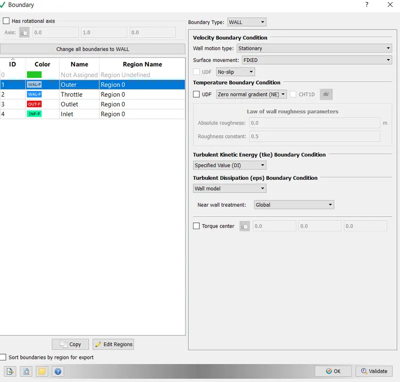
- Outer

4. Initial condition and events

The created geometry was selected as the Volumetric Region

5. Physical Models:- Default retained
6. Turbulence Modelling:- RNG-epsilon turbulence model is used
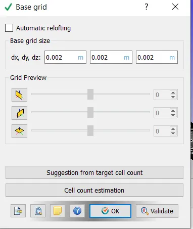
7. Grid Control:- A Grid size of 0.002 is entered in the dx, dy , and DZ direction

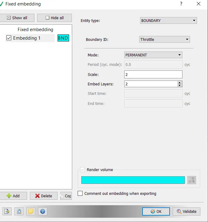
Fixed Embedding was also enabled. This was done to capture the flow around the throttle valve with greater precision. Scale 2 would mean that the size of the mesh at the throttle region would be reduced by four times.

7. Output/Post Processing:- The variables that we intend to see during post-processing are selected. In this case, Density, Pressure, Temperature, and Velocity were selected.

After setting the above, the input files were exported to a directory

In order to execute the simulation, the directory in which these input files were stored was accessed in Cygwin and the following command was typed "mpiexec.exe -n 4 converge.exe"

After the Simulation was executed, the results were converted into a form that would be compatible with Paraview. This was done using the post_convert.exe command.

Results:-

Surface with Mesh

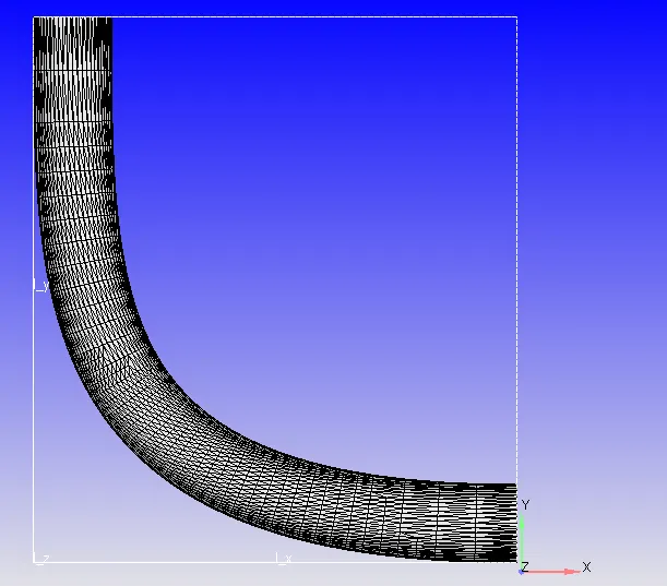
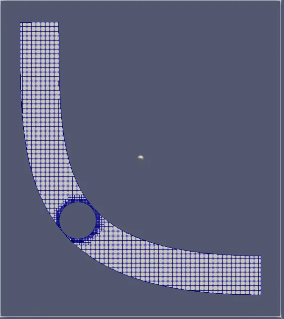
1) A Slice cut out with normal in the Z direction is given below. A fixed embedding scale factor of two was used which means that the cell size around the throttle would be 0.0005. This is done with the intent to capture finer details of the flow

2) Velocity Contour:- The velocity profile at various time steps is given below.

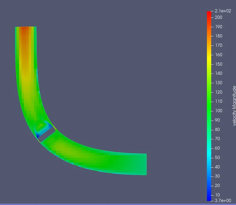
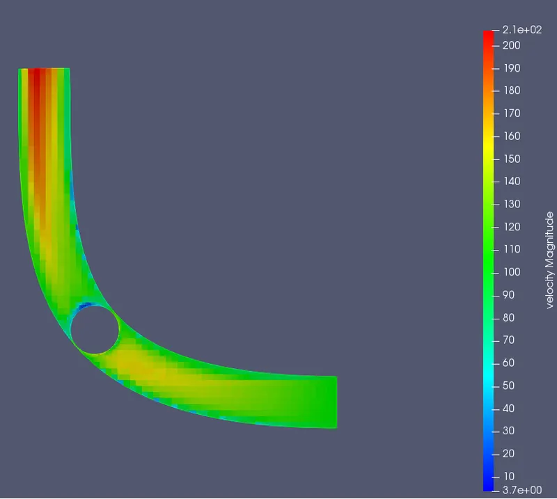
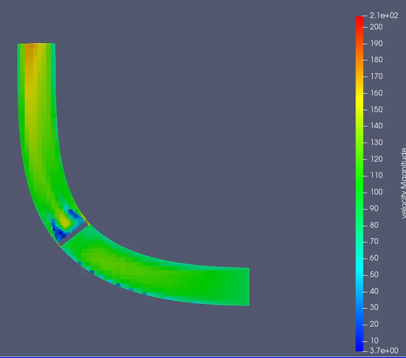
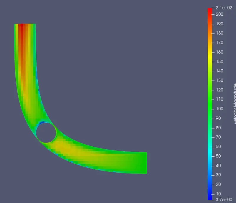
From the contour plots, it is noted that the movement of the throttle valve has a bearing on the outlet velocity. The maximum velocity is achieved when the throttle is open, ie it is aligned/ parallel to the flow direction.

2) Pressure Contour:- Plot of Pressure contours is given below at various time steps

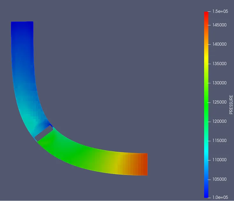
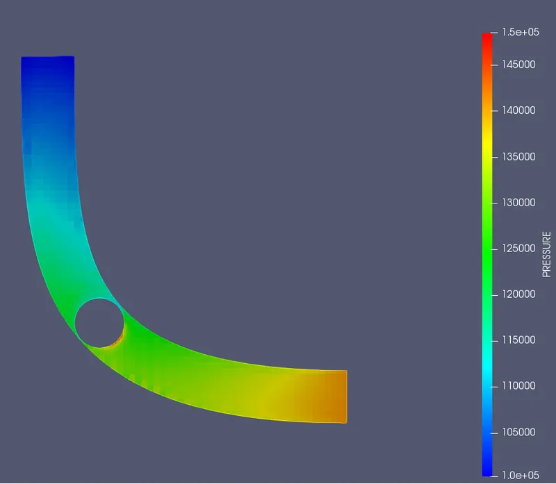
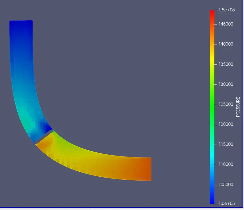
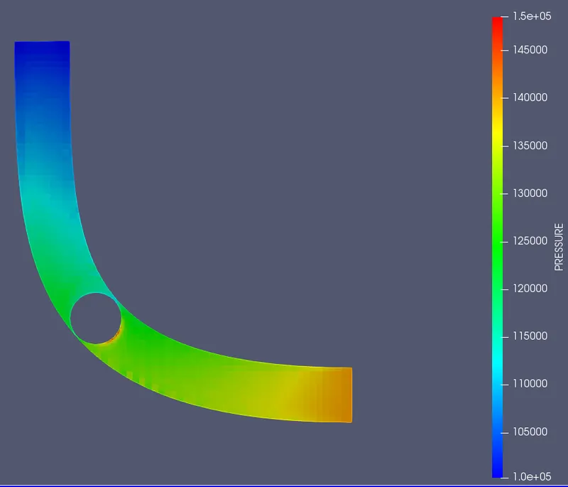
It is noted that the movement of the throttle valve has a bearing on the outlet pressure. When the valve closes it is observed that two distinct pressure zones are created.

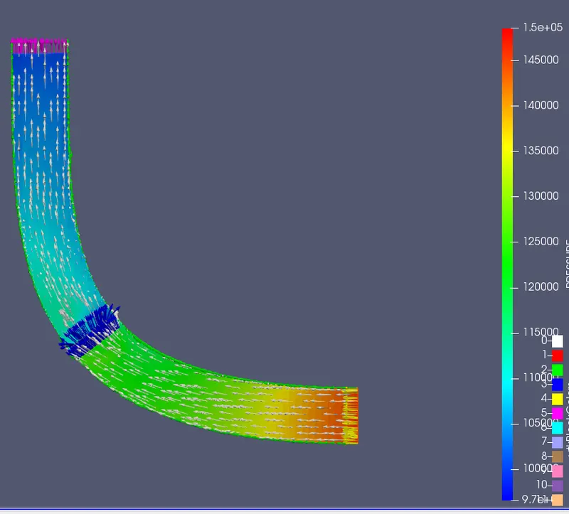
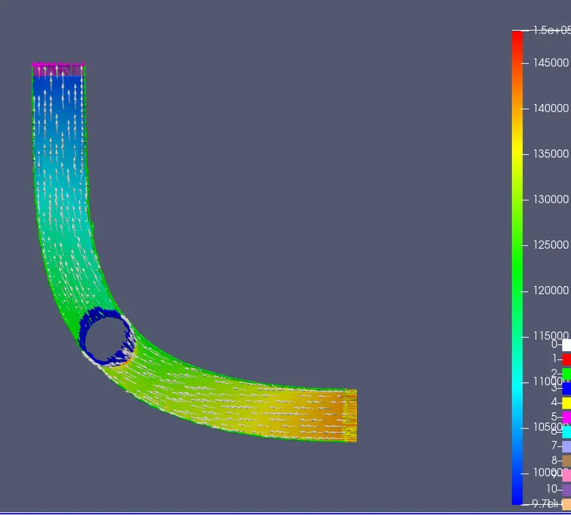
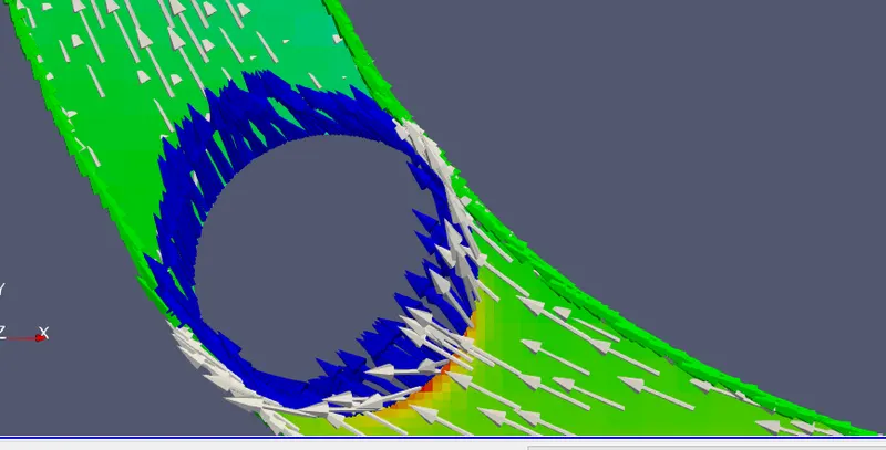
3) Velocity Vectors

Valve in closed position:-

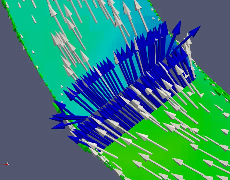
-Valve in Open Position

Plots.

i) Mass Flow Rate

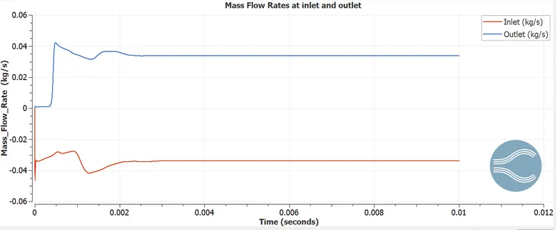
From the above plot, we note that the mass flow rates at the inlet and outlet initially vary until 2 milliseconds after which they attain a constant value of 0.35 kg/s for the rest of the simulation

ii) Average Velocities

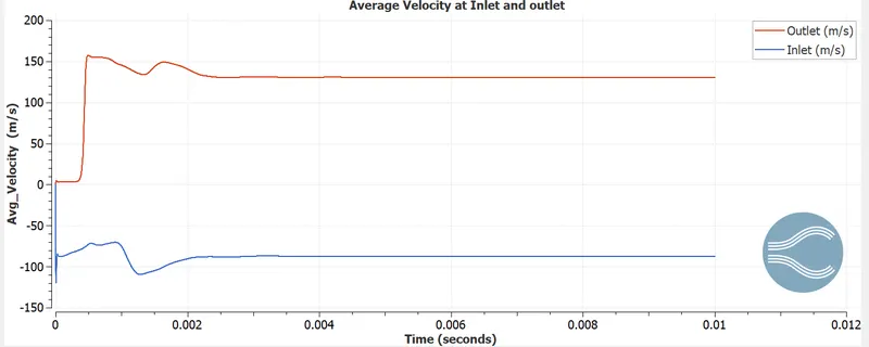
The average velocities to exhibit a similar trend to the Mass flow rate. Until 2 milliseconds, there is a variation after which it attains a constant velocity of around 150 m/s

iii) Total Pressure

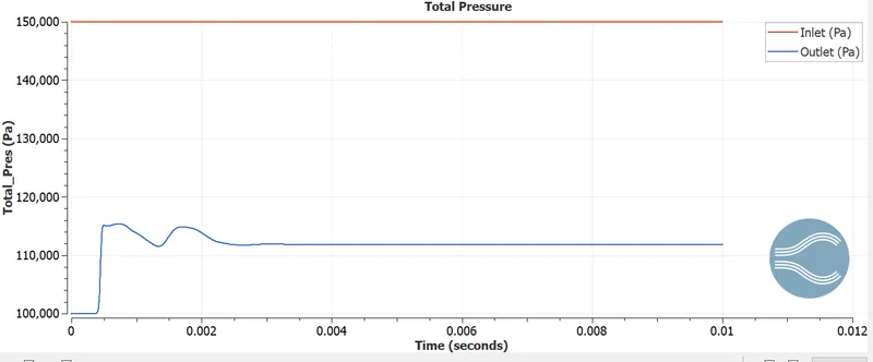
From the above plot it is seen that while the inlet pressure is constant at 150000 Pa, the outlet Pressure reaches a value of a little below 114,000 Pa after 2 milliseconds

iv) Cell count

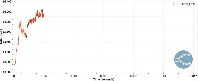
Cell count initially varies until 2 milliseconds. This can be attributed to the movement of the throttle valve from 0 to 25 degrees until 2 milliseconds.

Calculation of Simulation end time

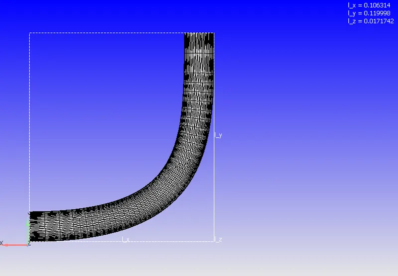
Characteristic length is 0.106 m, say 0.11 m

The average velocity at the inlet is around 80m/s for steady state (from previous assignment)

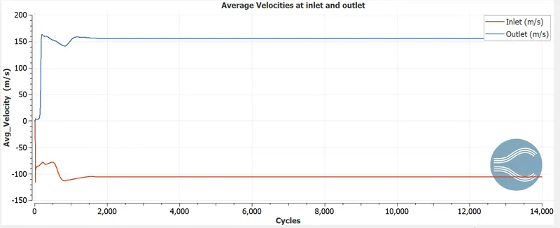
Flow through time = 0.11/80=0.0013 seconds say 0.002 seconds or 2 milliseconds for fluid to flow once through the pipe. We intend to simulate 5 such movements therefore an end time of 0.01 seconds is chosen.

Animation showing the Movement of the Throttle Valve

Development of Velocity Profile

Conclusion

In this analysis, transient simulation is studied. Through contour plots for velocity and pressure, it is observed that the movement of the throttle impacts the velocity and pressure in the region rear to the throttle valve. Also, movement of the throttle has an impact on the cell count until 2 milliseconds.