Week 4.2: Project - Transient simulation of flow over a throttle body

Aim : Transient state simulation of from over throttle body using Converge Cfd.

Objectives:

• Set a case for transient floe in converge Cfd.
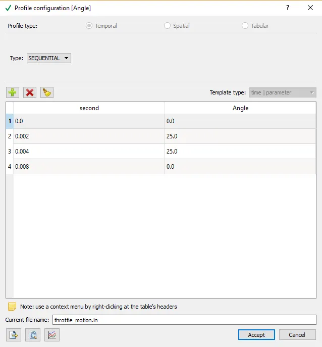
• Throttle rotation rate:

1. At 0 : 0 degree
2. 0 to 2ms : 25 degree
3. 2ms to 4ms : 25 degree
4. 4ms to 8ms : 0 degree

• Post process in paraview and provide detailed explanation for case with contours, and animation.

Introduction:

Transient flow :

The change of parameters not only depends on location but also on time. It is also called as unsteady flow.

As we rotate the throttle since its changing its position there is change of flow parameters with respect to time which we can be calculated using transient state solver in converge Cfd.

Steps that should be changed in case of transient flow:

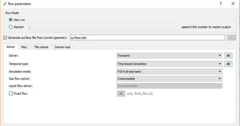
• In run parameters we should select transient solver with temporal type as Time-based simulation.

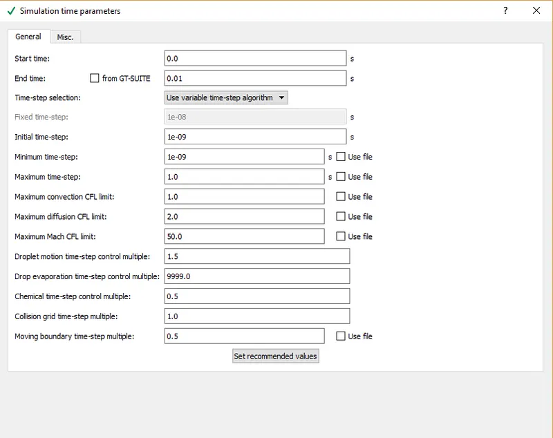
• In simulation time parameters, we can control start time-end time and time steps also CFL number which actually controls the stability of any solution.

To calculate time step we can take a value of average velocity we get from steady state simulation, and multiply it with length of the elbow we get time taken by air to pass elbow, and then we can mutiply the value with any factor 'n' to get required number of iterations.

Assume,

Average velocity = 200 m/s

length = 0.2 m

Then, time taken(t) = distance(L) / velocity(v) = 0.2/200 = 0.001s

No of iterations = n * t = 10*0.001 = 0.01s

End time = 0.01s

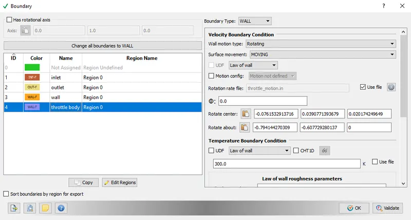
• In boundary condition the only change is done to throttle body which is taken to be rotating/moving body with a file to add the rotation parameters, and need to fill arc center and arc normal points to define axis of rotation.
• To calculate rotate about and rotate center we can use ( measure-> arc normal) select any three points on the circle and apply we will get values for above in message log we can copy and paste it.

RESULTS:

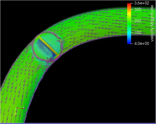
Glyph:

The flow direction can be seen from inlet to outlet.

Velocity Contour:

Pressure contour:

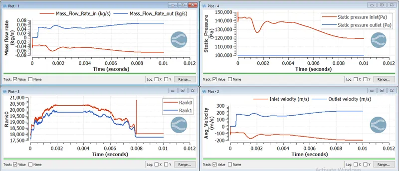
Plots for mass flow rate, avg velocity, cell count and pressue:

Link to the video:

https://drive.google.com/file/d/1q_TDE7cSNaAKdxFQ3eJmC8G1WHBC5Bqp/view?usp=sharing

Conclusion:

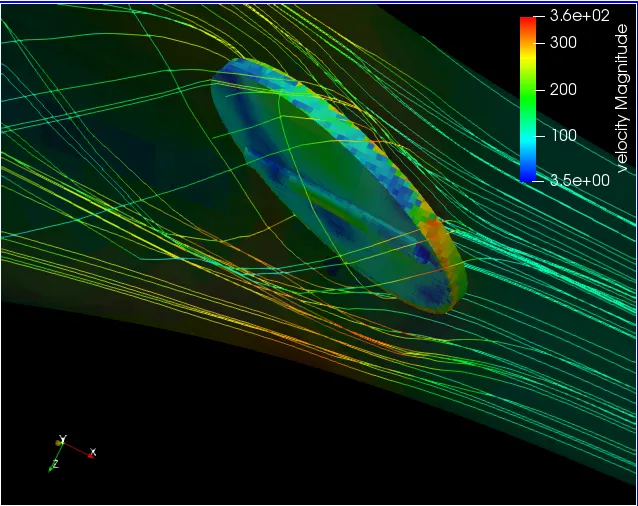
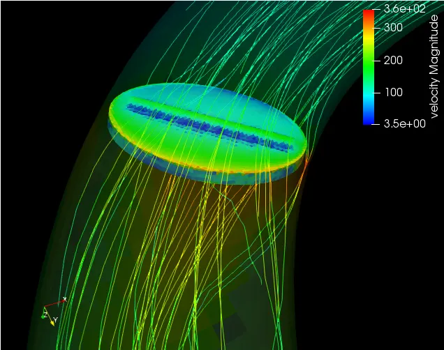
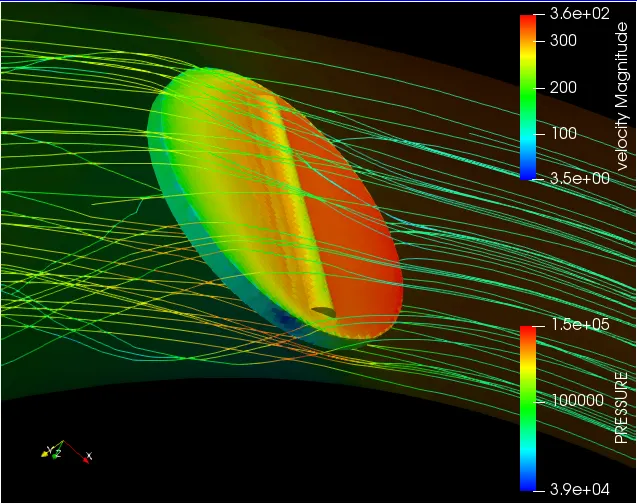
• From the pressure and velocity contour it can be seen that at high pressure region the velocity is low, which is obvious case as the air hits the throttle at inclination pressure increases and velocity retards.
• The mass flow rate, velocity, pressure varies continously as the wall rotates.
• The cell count also varies as the throttle rotates and adapt itself to the new position of throttle this provide flexibility in simulations.