Challenge

Week 4.1 - Solving second order ODEs

DDeepan M R24 May 2024

SOLVING 2nd ORDER DIFFERENTIAL EQUATIONS- 1 DOF PENDULUM

AIM

Understanding the use of ODE45 function in solving a differential equation
Plot the results and save the results into an animation video file

THEORY

The pendullum system considered here has a mass and a damping also the effect of acceleration due to gravity.
The differential equation of the system is as follows

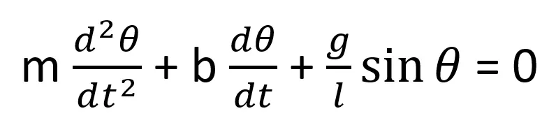
m is the mass of the bob

b is the damping constant

g is the acceleration due to gravity

l is the length of the pendullum

Numerical methods are used to solve differential equations. In matlab here we use ODE45 function to solve this equation which adopts Renga-Kutta method of 4th order for solving and RK method of 5th order for error calculations.

Finding the position of the pendulum is very much important in the design of pendulum.

PROCEDURE

clear

close

clc

% Length of the pendulum in m

l=1;

% g is acceleration due to gravity in m/s^2

g=9.81;

% b is the damping constant in Ns/m

b=0.05;

% m is the mass in kg

m=1;

% Initial ang. displacement = 0 and angular velocity = 3

initial_angle_vel = [0;3];

% time spans from 0 to 100 with dt = 0.1

t_span = 0:0.1:100;

% ODE45 is the solver used t stores the time and results stores the ang.

% displacement and ang velocity

% t, theeta stores the current value of time and time, angl displacement

% and angular velocity

% odefunc is a function calling which calls the function

% It calculates the requires function definition or simply it calculates and stores the differential value

[t , results] = ode45(@(t,theeta)odefunc(t,theeta,b,g,l,m),t_span,initial_angle_vel);

figure(1);

% First column gives the angular displacement

plot(t,results(:,1),'LineWidth',2,'Color','r');

% hold on is used to incorporate the next plot in the same figure

hold on

% Second column data gives the angular velocity

plot(t,results(:,2),'Color','b','LineWidth',1);

xlabel('Time');

ylabel('Plot');

legend('Angular Displacement','Angular Velocity')

% stores the angular displacement for every time step and makes it into a

% row matrix by transformation

angle = results(:,1).';

% use a for loop to calculate the length at every step

for i=1:length(angle)

x(i) = l*sin(angle(i));

y(i) = -(l*cos(angle(i)));

figure(2);

plot([0 x(i)],[0 y(i)],x(i),y(i),'o','MarkerSize',20,'MarkerFaceColor','g')

%plot()

title({'Pendulum Motion';'Initial angular displacement = 0 rad';'Initial Angular Velocity = 3 rad/s'})

xlabel('X-Position');

ylabel('Y-Position');

xlim([-1.1 1.1])

ylim([-1.1 1.1])

pause(0.03)

% used to capture the individual frames

video(i) = getframe(gcf);

end

% collecting the frames

movie(video)

% creating the video file and assigning it to a variable file

file = VideoWriter('pendullum.avi','Uncompressed AVI')

% opening the video file

open(file)

% write the frames in video to the file created

writeVideo(file,video)

close(file)

function[dy_dt] = odefunc(t,theeta,b,g,l,m)

% theeta_1 stores the value of displacement

% In first calculation it will hold the initial condition

theeta_1 = theeta(1);

% theeta_2 holds the velocity data

theeta_2 = theeta(2);

% Rate of change of displacement gives the velocity

dtheeta1_dt = theeta_2;

% this is the equation of acceleration

dtheeta2_dt = -(b/m)*theeta_2 -(g/l)*sin(theeta_1);

dy_dt = [dtheeta1_dt ; dtheeta2_dt];

end

RESULTS

The angular displacement and angular velocity of the pendulum is found out and plotted against time
The position of the pendulum is plotted and the plots are animated and exported as a video file
The code is set for 100s it can be changed to 20 seconds also

VideoFile

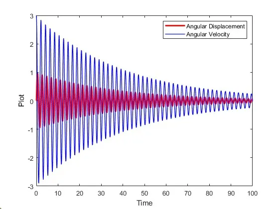
Plot of Ang velocity and displacement v/s time

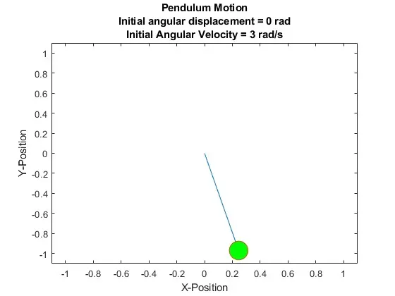
Spacial position of the pendulum

Week 4.1 - Solving second order ODEs

Ship work like this
in your own course.

Talk to a career counsellor

Ship work like thisin your own course.

Talk to a career counsellor

Ship work like this
in your own course.