Week 2 - Flow over a Cylinder.
Karman Vortex Street
PART 1
Aim
Flow simulation to study Karman Vortex shedding
Introducation
- Air (User-defined material) is allowed to pass over the cylinder
- Reynolds number is varied by adjusting the dynamic viscosity for the simplicity of the analysis
- For the Part 1 we use steady state and transient state simulation with laminar viscous model and a Reynolds number of 100
Theory
- Under certain flow conditions, the flow around a buffed body can result in vortex-shedding even in laminar flow and the phenomenon is known as Karman Vortex Street
- The freequency of this vortex is of prime importance as this can result in catastropphic damages to structures if the freequency becomes equal to fundemental freequency(reosonance)
Procedure
- The working domain is chosen as Fluid Flow (Fluent)
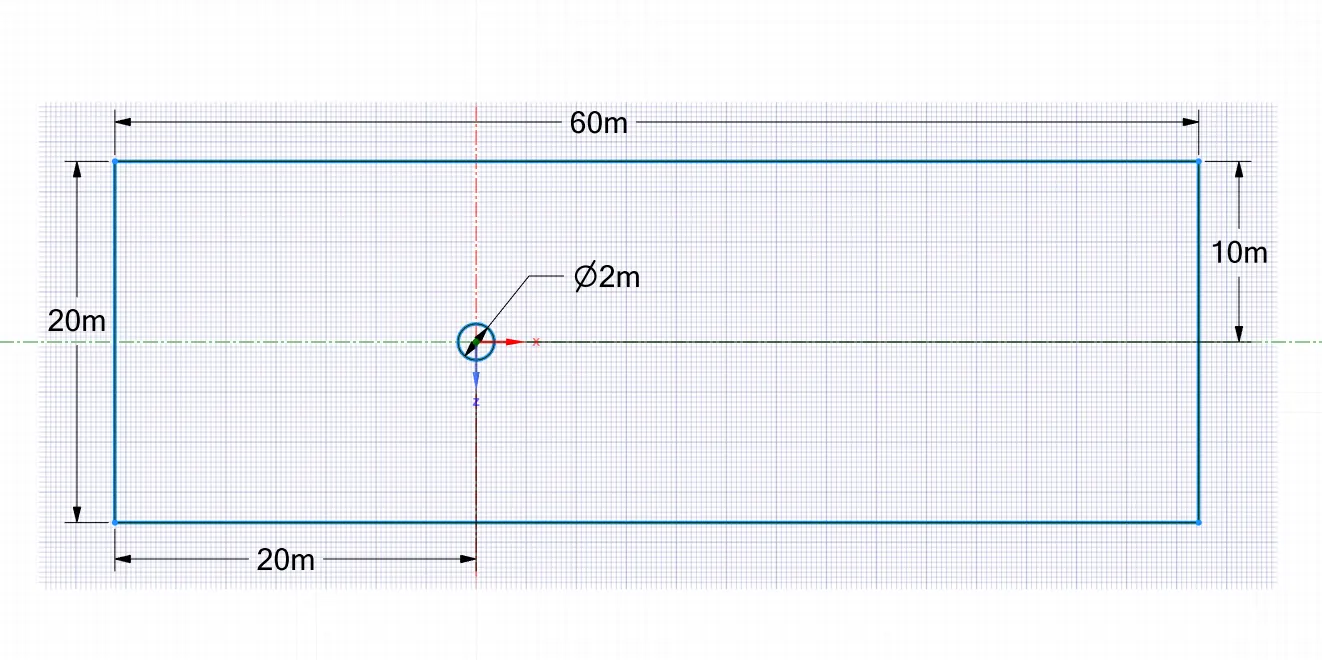
- For geometry creation we use space claim and draw and complete the geometry as shown below
- Upstream 10 D, Downstream 20D, Height 10D (D=2m)
- Convert the sketch to a suface by pull option
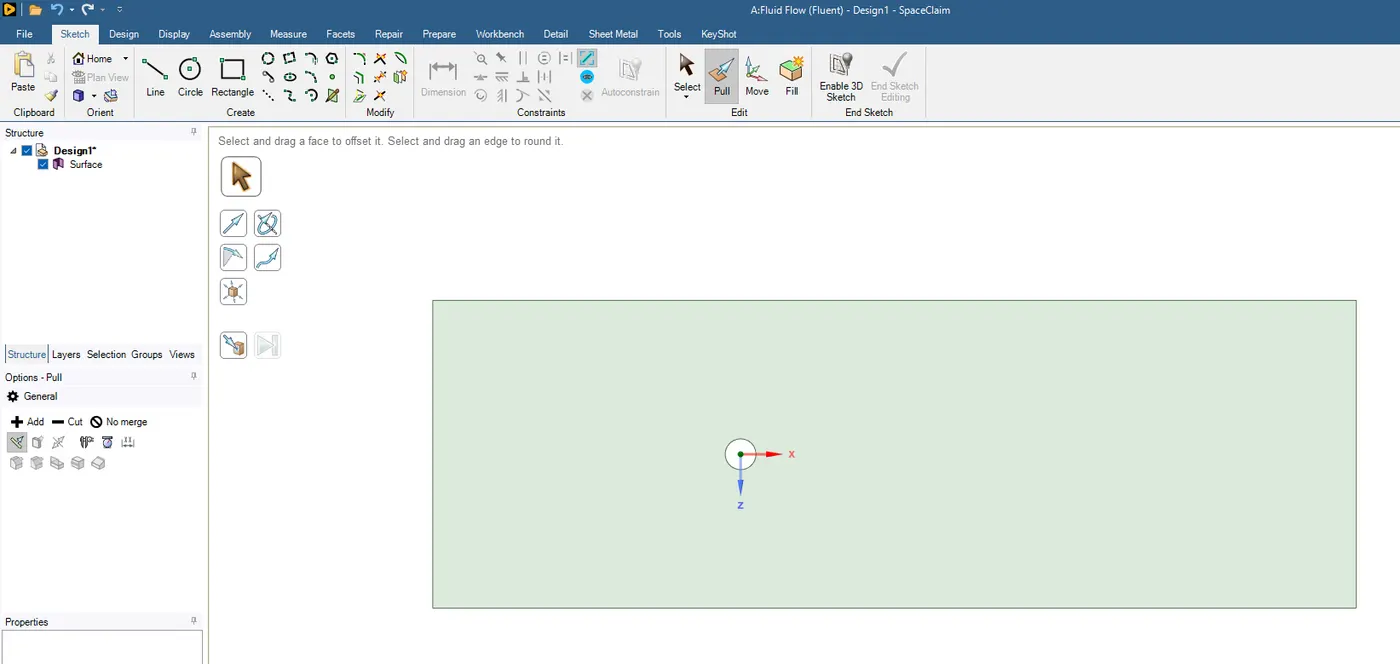
- In the mesh, generate the mesh
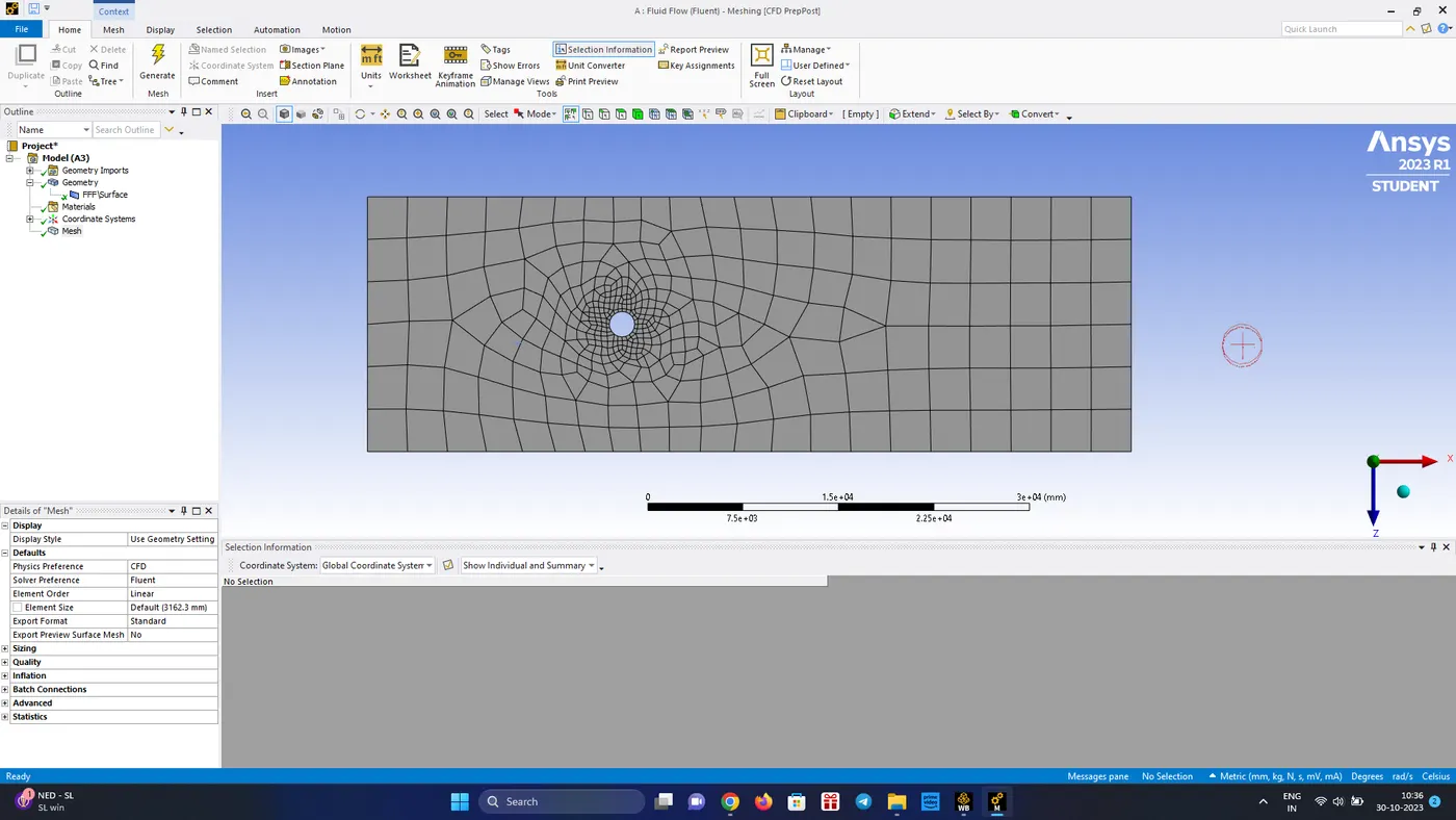
- Change the meshing methods and change the element type to triangles.
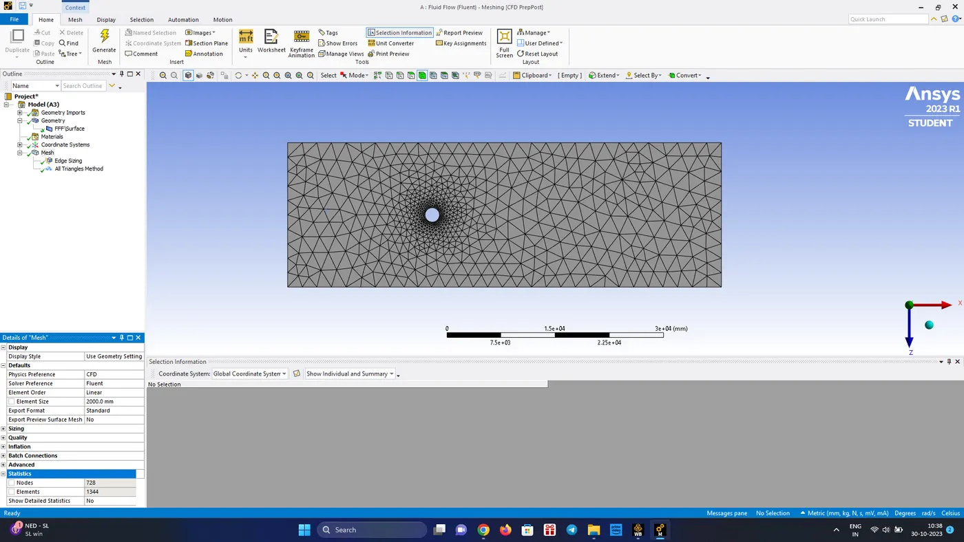
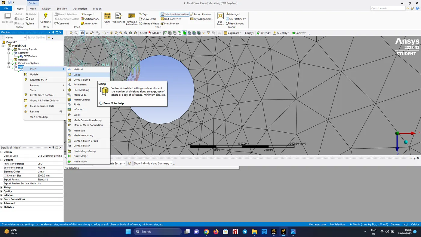
- For the cylinder we can see that it is not well defined
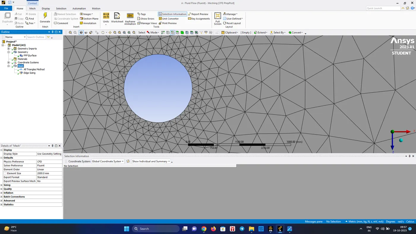
- Insert ----> Sizing ----> In the geometry click the edge Apply ----> Change the type to Number of divisions and use 36 divisions and click generate mesh.
- The mesh quality is improved
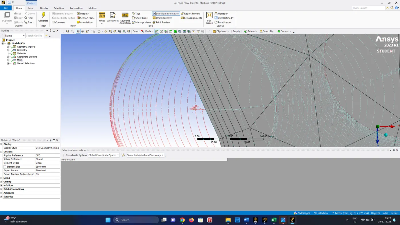
- Introduce inflation 6 inflation layer around the cylider to acurately capture the geometry and to get body fitted mesh (first layer thickness 5mm and growth rate 1.2)
- Change the mesh element size to 250 mm
Nodes: 20710
Elements: 40528
- Name the inlet, outlet and cylinder walls and the upper and down portion as symmetry
- Open Setup
- Check for mesh quality check and make sure all the parts are imported also check for namings in boundaries
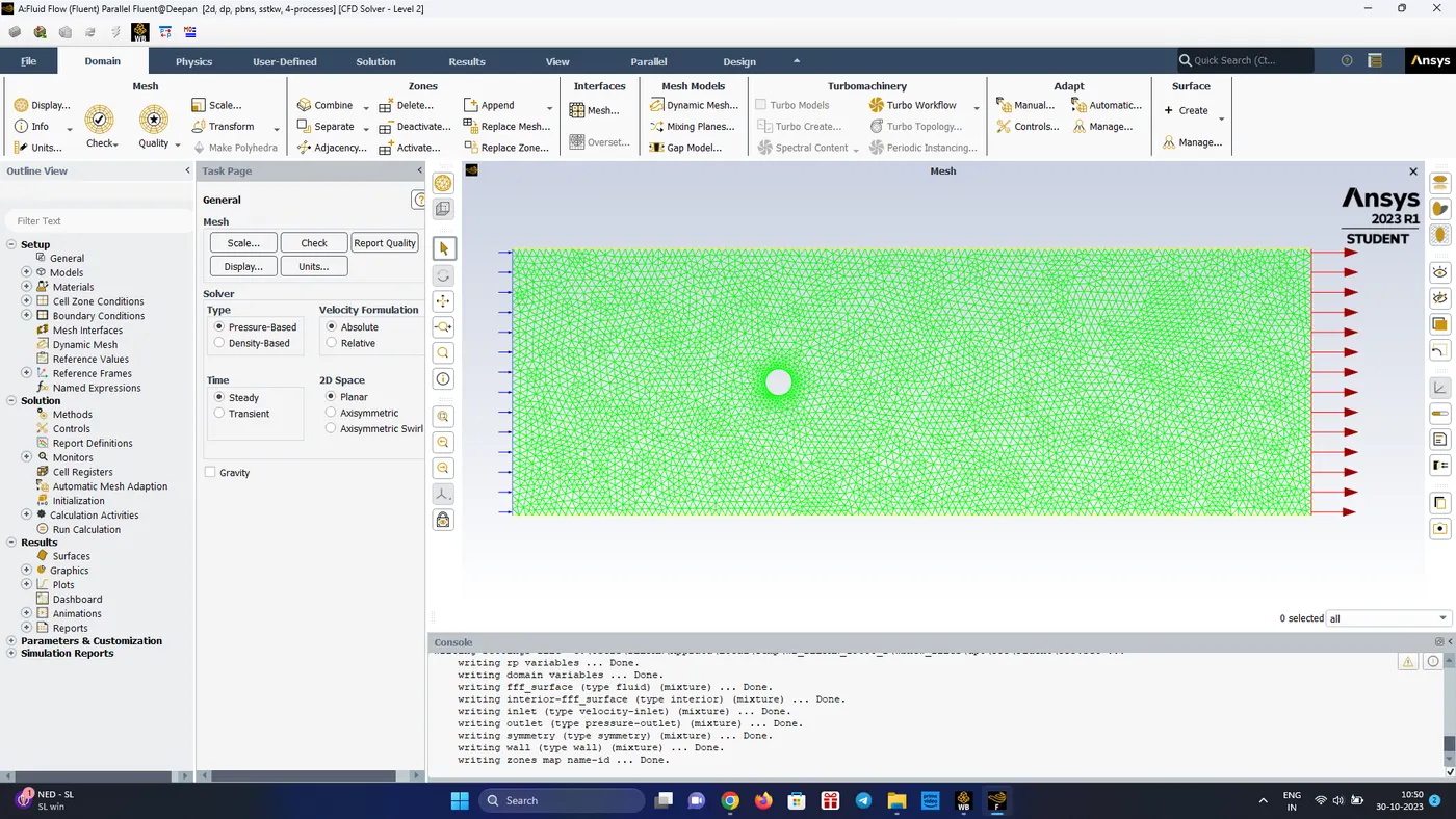
Solver:
- Type: Pressure-Based
- Velocity formulation: Absolute
- Time: Steady
- 2-D Space: Planar
- In the Physics choose the viscous model as laminar
- Materials(Create/edit) ----> Fluent Database ----> Air ----> Copy
- Save as User-Material and change the material density as 1 kg/m3 and viscosity as 0.02 kg/ms -----> change/create
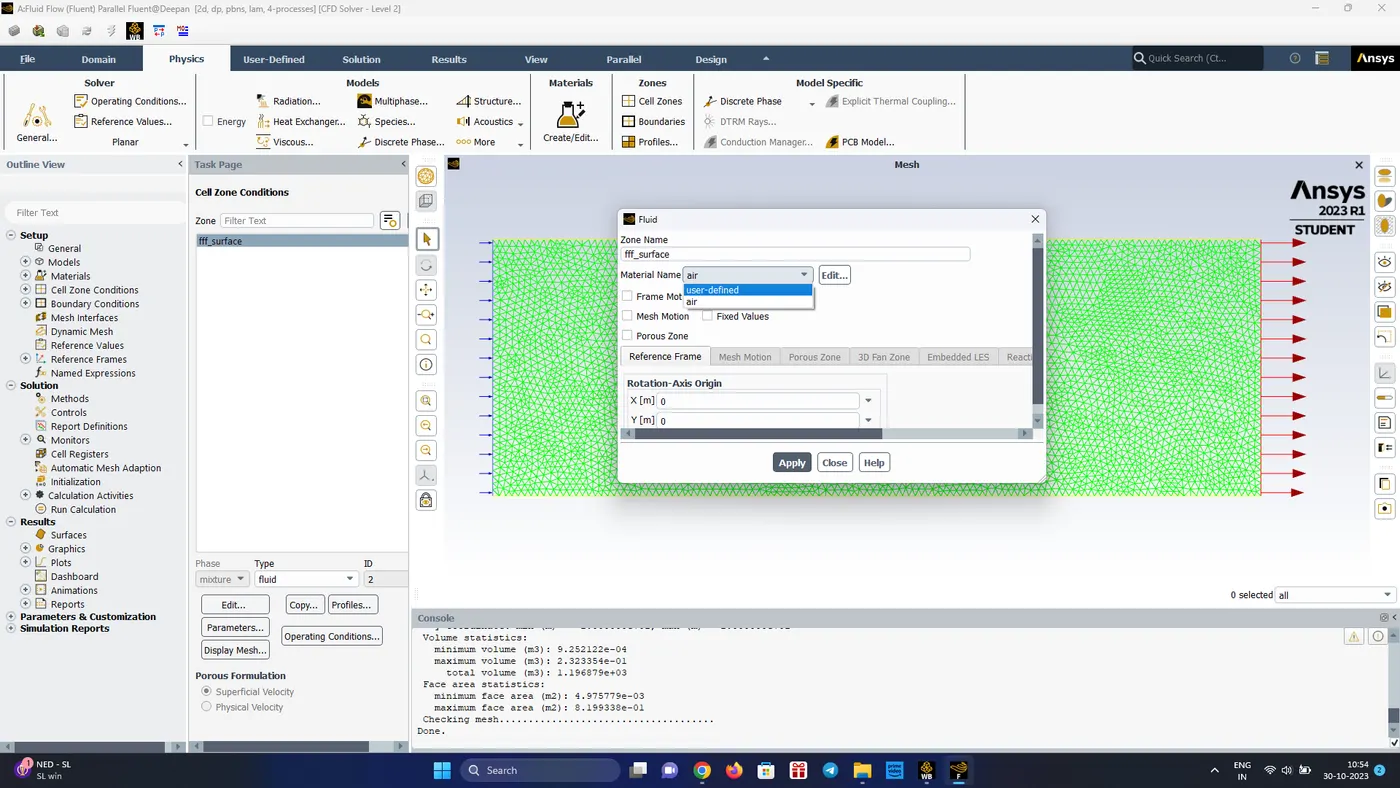
- In Zones -----> Cell Zones ----> Change the material to usser-defined
- In the materials delete the default fluid material
- In the residuals, uncheck the convergence criteria
- Then we need to create a monitor point, which is 4D-5D from the cylinder, here we take the monitor point to 5D (10m)
- The average vertex velocity magnitude at the monitor point help us in concluding whether the flow has achieved convergence or not.
- In addition to this in the definitions ----> Force reports ----> Add drag and lift
- In the reference value change the area to 2 sq.m and change the viscosity and density.
- Initialize the problem with hybrid initialization and use SIMPLE method for solving
- In the results add velocity contour plot and in the solution activities add solution animation for velocity contours
- solve for 350 iterations
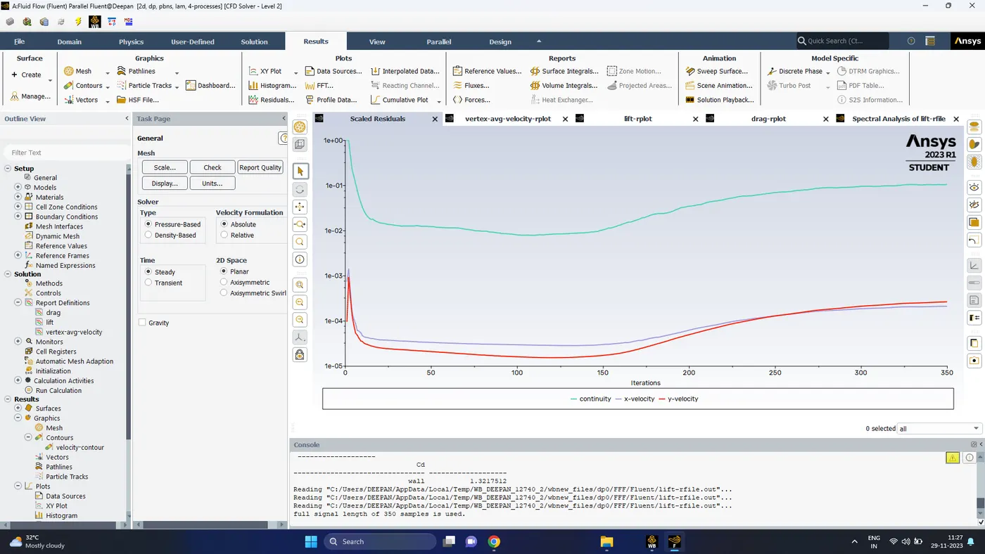
Scaled Residuals
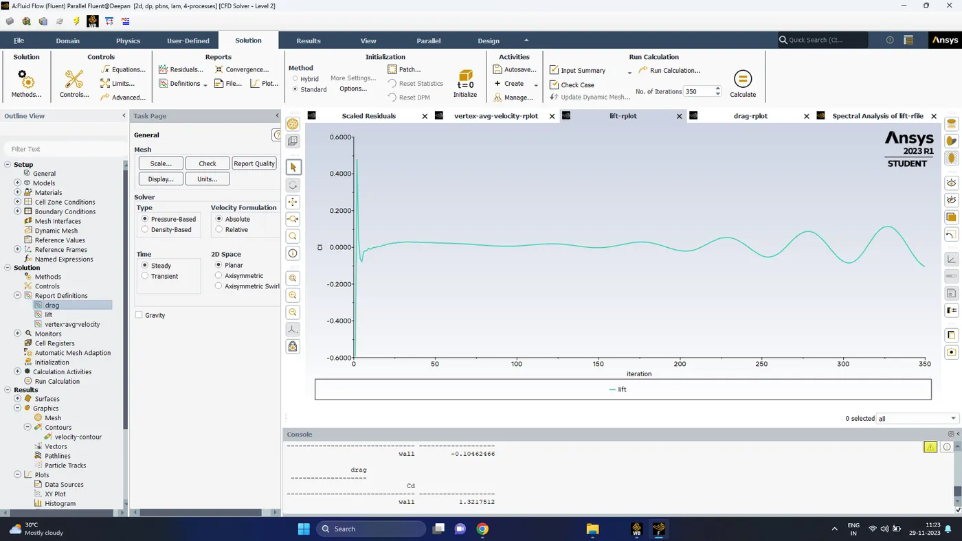
Co-Efficient of Lift (-0.104)
- The fluctuation is seem to start at around 110 to 120 iterations and it seem to increase, which indicates that the solution is not converged
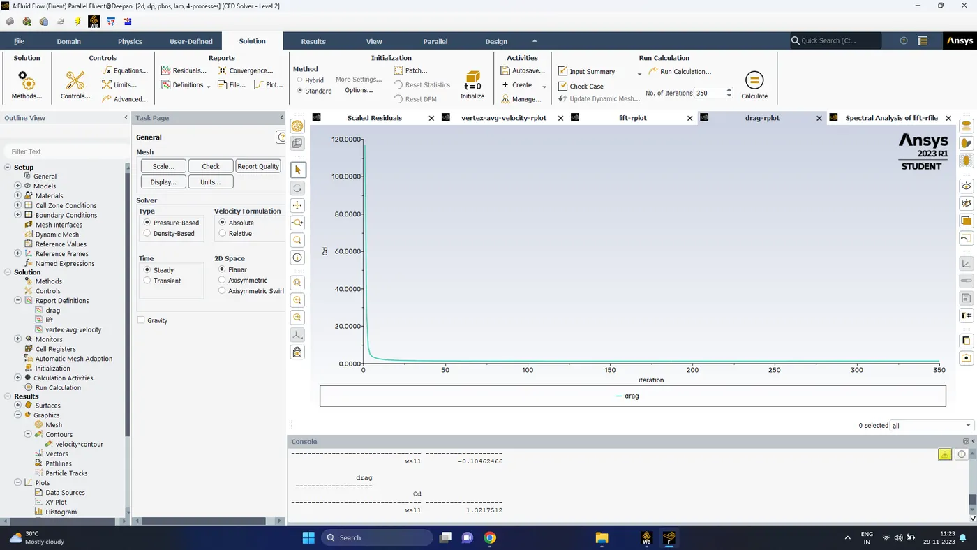
Co-Efficient of Drag (1.321)
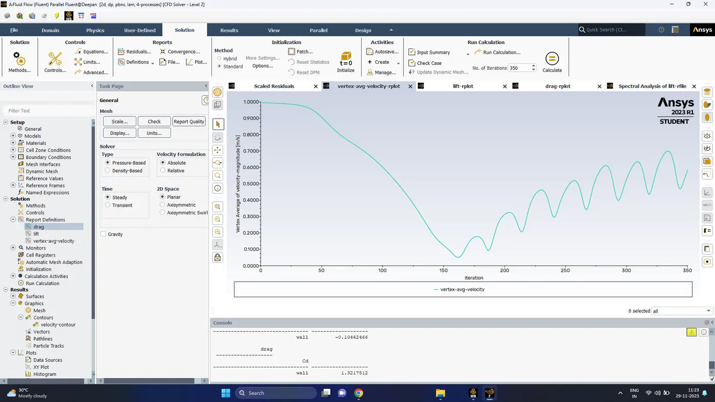
Vertex Avg of Monitor Point Velocity
- A disturbance in general velcity trend can be observed at around 160 iterations
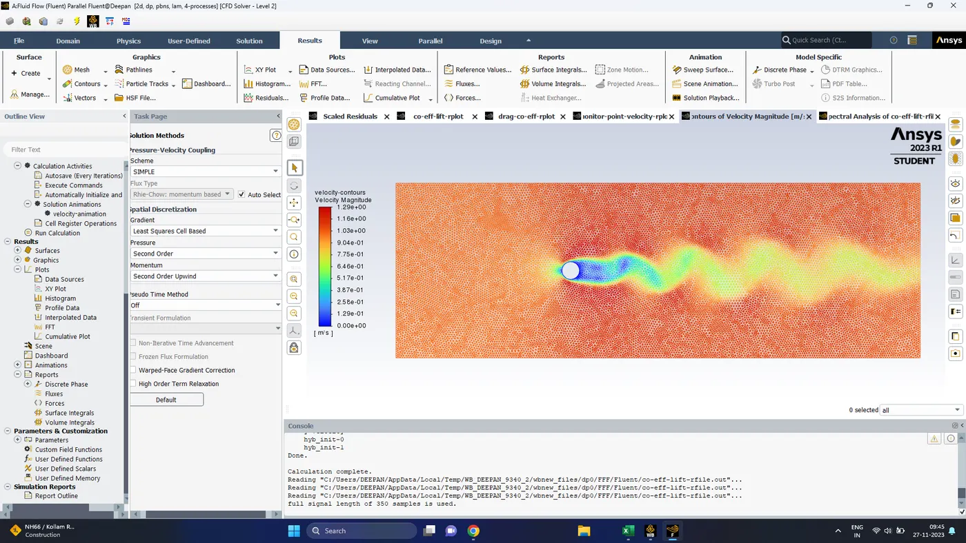
- In the velocity contours we can clearly see the vortex shedding
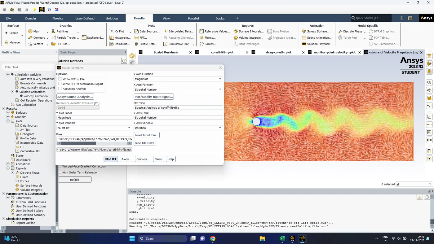
- The next step is to find the strouhal number which relies on the lift co-efficient plot and its freequency
- In the results ----> FFT----> Y-axis function change to magnitude ----> then load the lift co-efficient function and plot the graph
- The peak of the graph and the corresponding strouhal number will be taken as the strouhal number
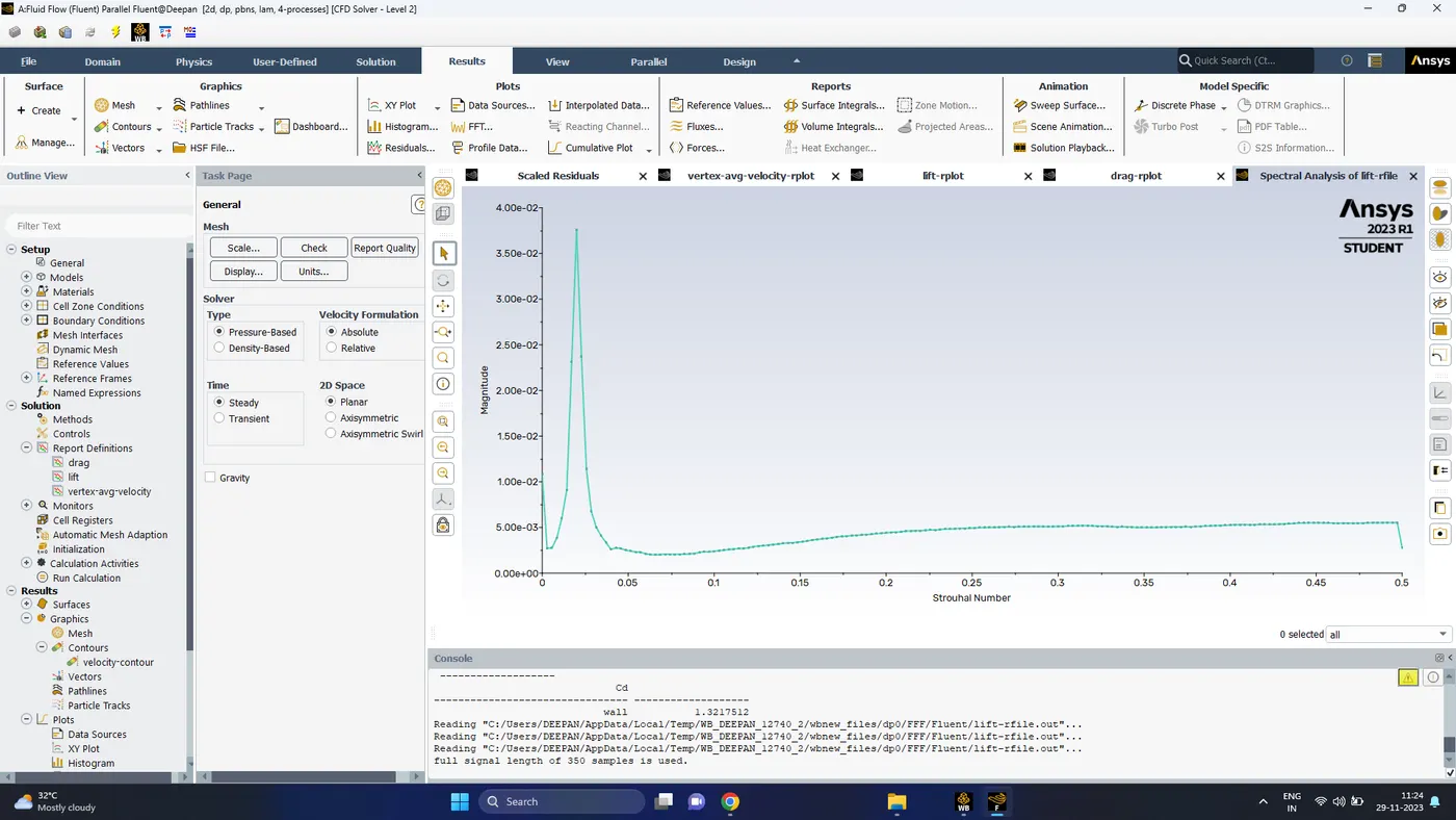
The strouhal number is obtained as 0.0203
To achieve convergence, the solution is continued for 1000 iterations.
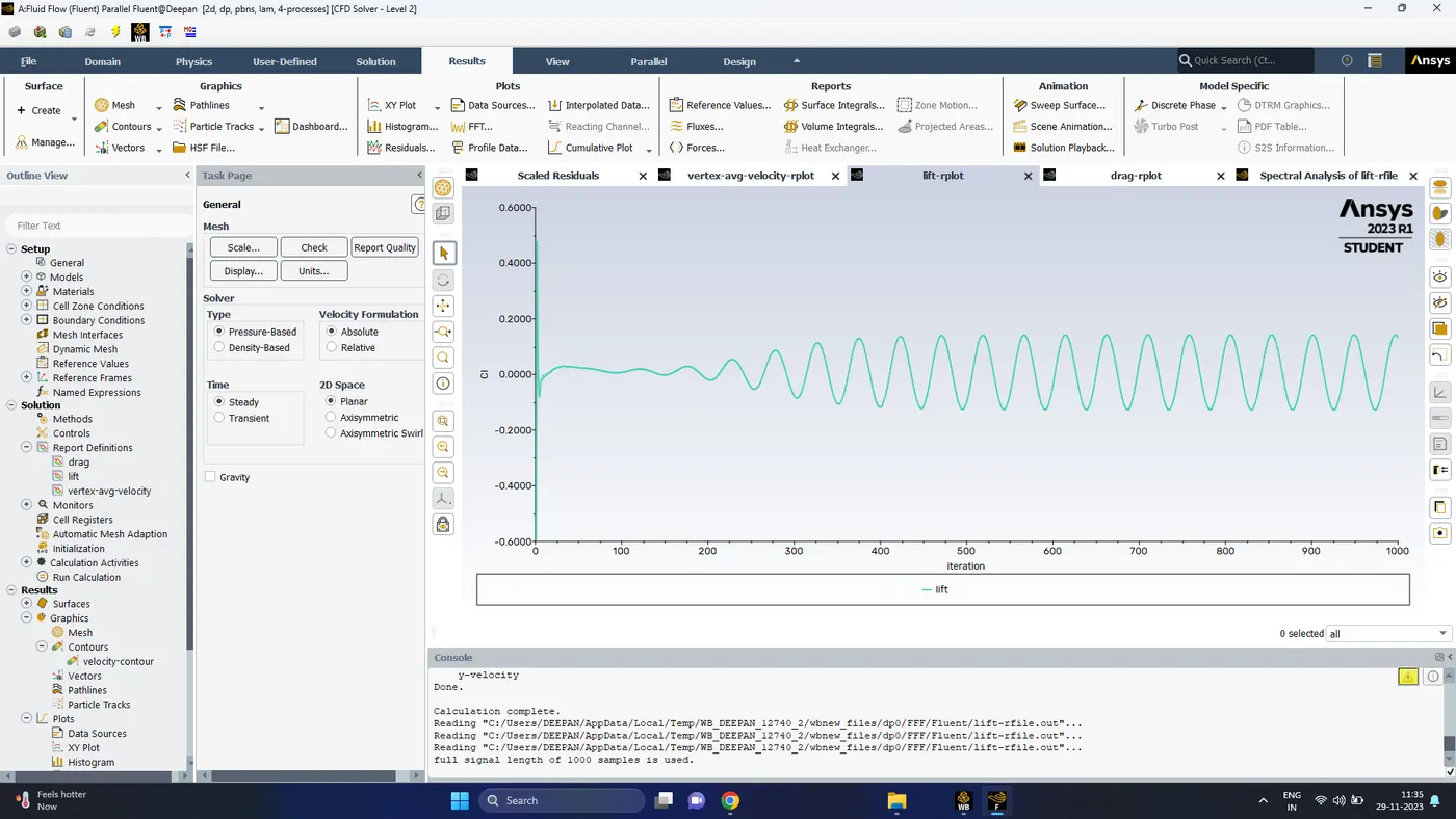
Co-efficient of Lift (1.328)
- We can see a general repeating pattern with a fixed freequency, which indicates the solution has achieved convergence
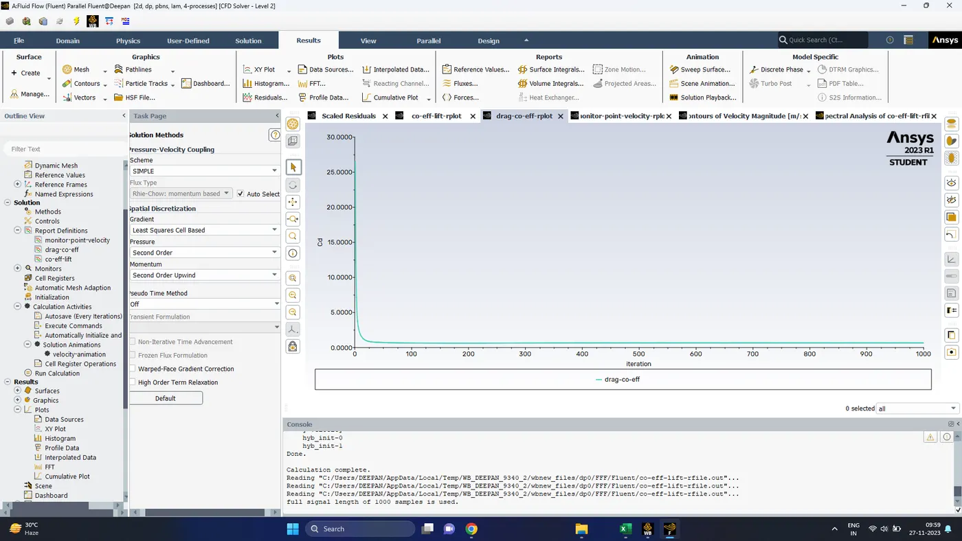
Drag Co-efficient (1.34)
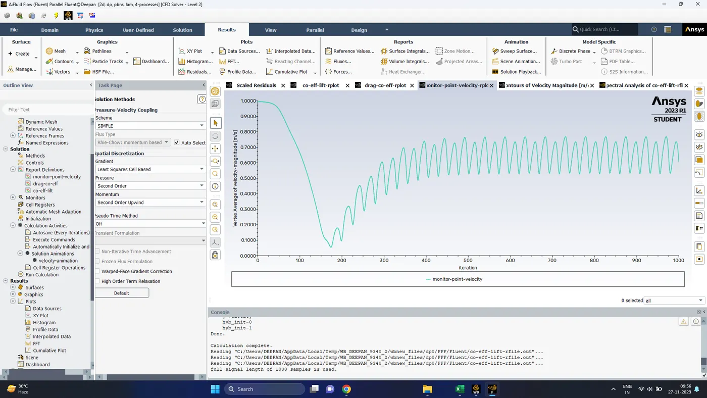
Monitor point Velocity
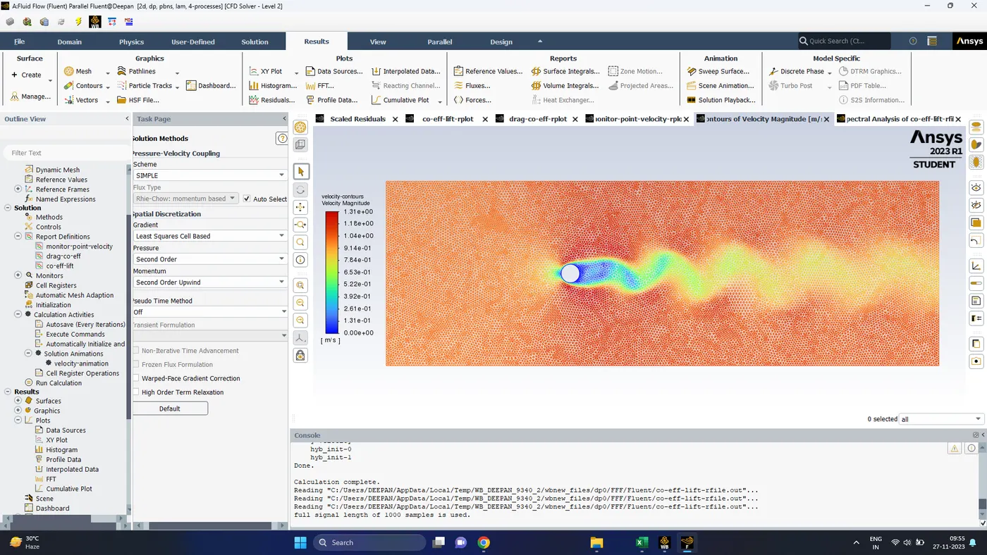
Velocity Contours
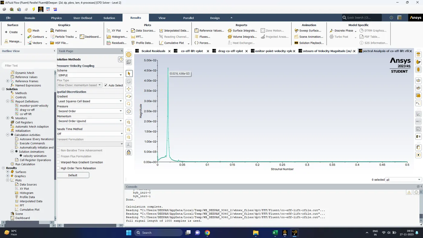
Strouhal Number = 0.0216
Transient-State Analysis
Time Step Size: 0.1s
Number of Time Steps: 500
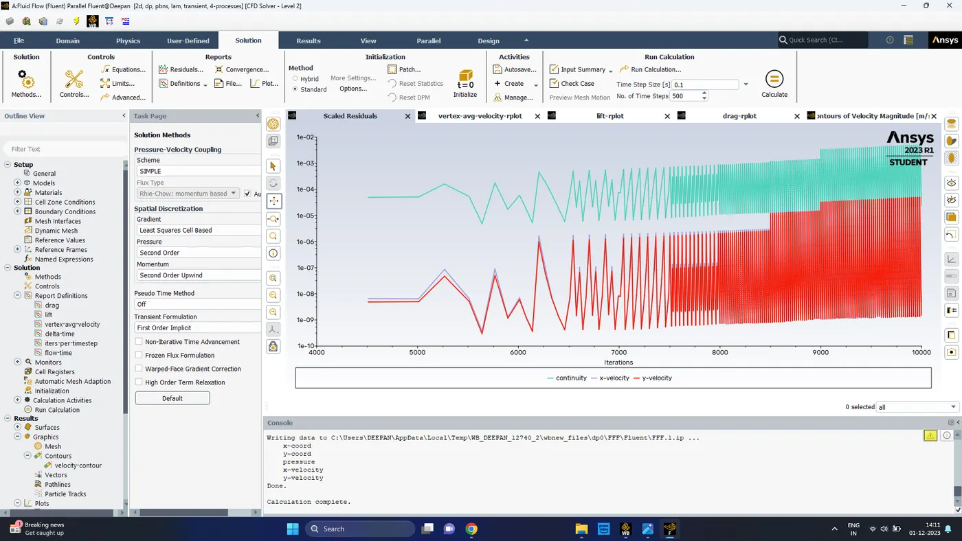
Scaled Residuals
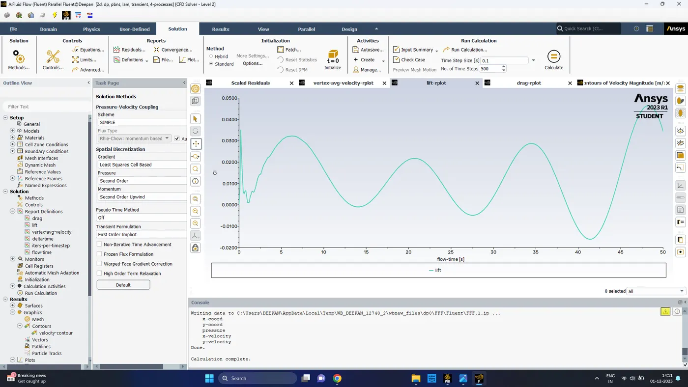
Lift co-efficient
- We can clearly see large fluctuations in the plot which are a clear indication of an un-converged solution
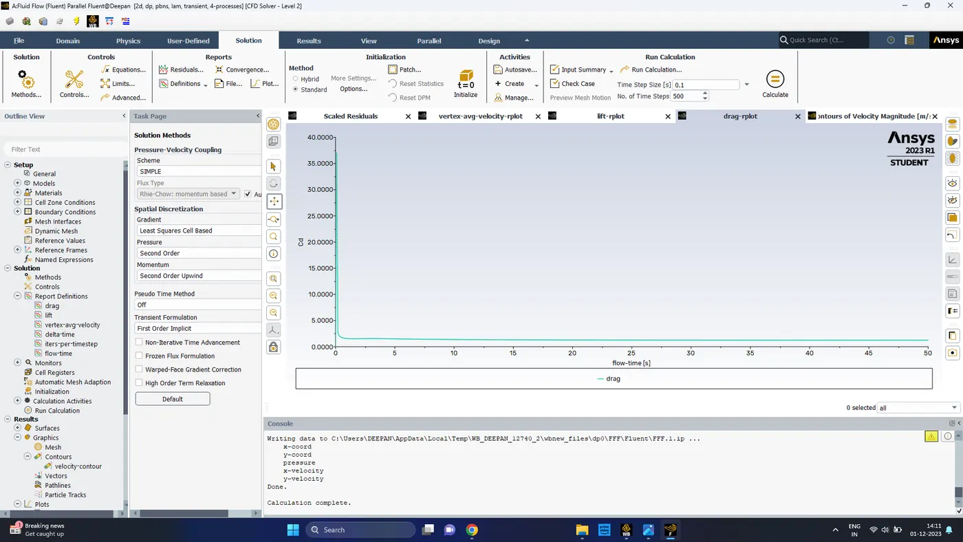
Co-efficient of drag (cd= 1.258)
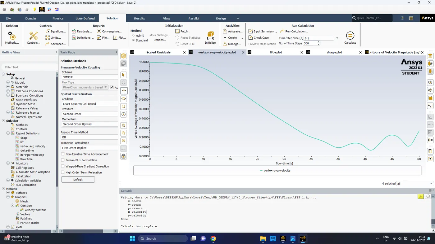
- The monitor point velocity started showing some vortex shedding at around 30s
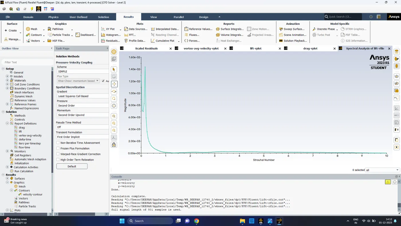
Strouhal Number (St = 0.16)
To obtain a better solution we run the solver for another 50s or 500 time steps
Time: 100s (1000 time steps)
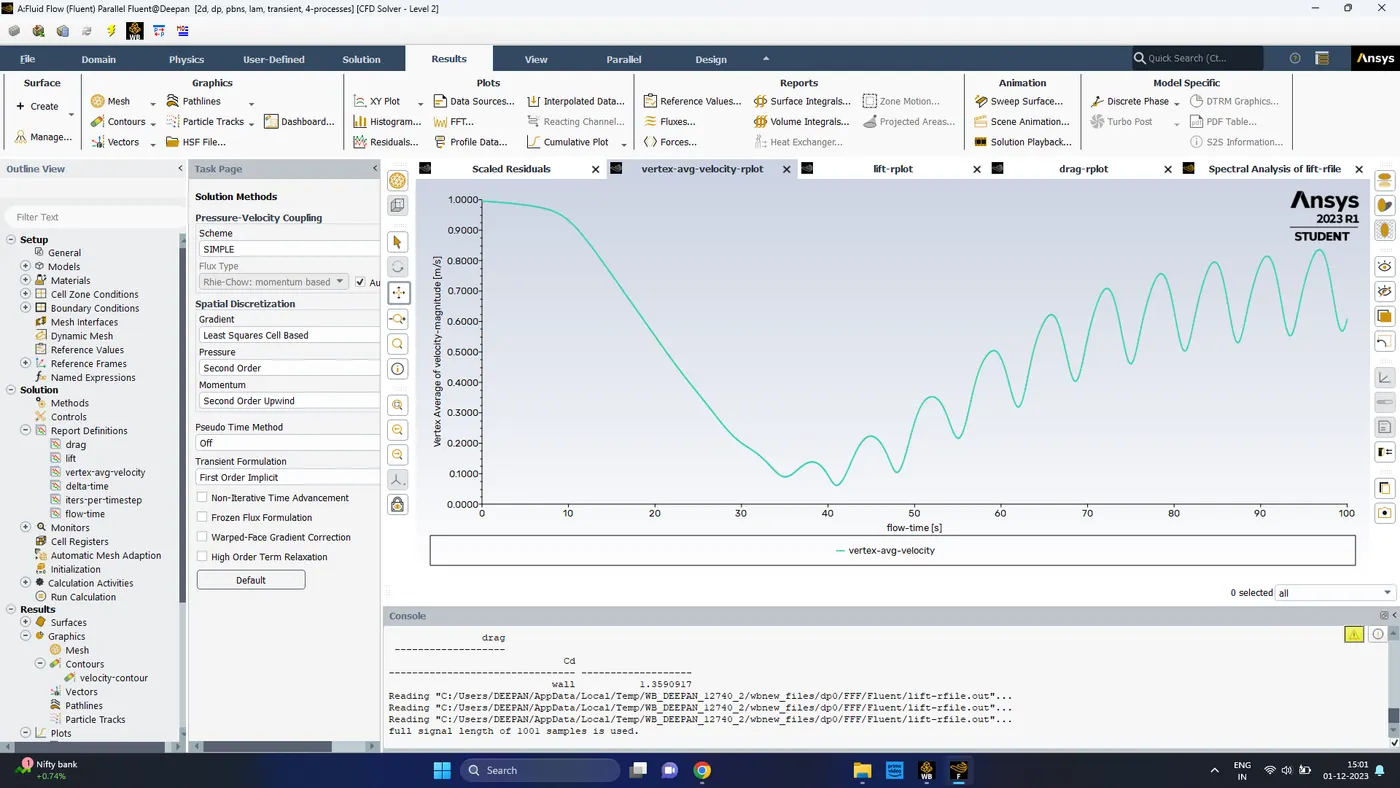
- The monitor point velocity is slowly approaching a steady repetitive pattern, indicating the flow is steadily attaining a converged solution
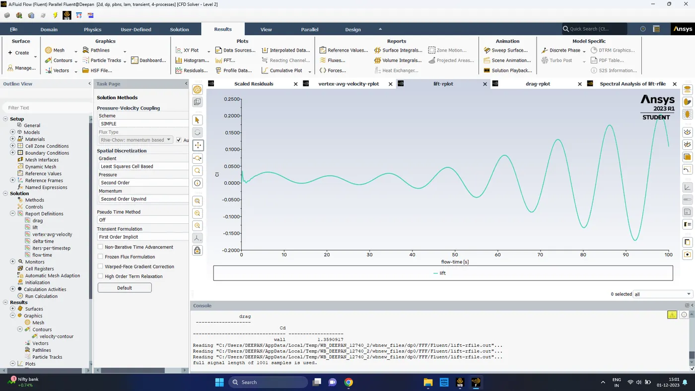
The plot of lift co-efficient is still developing, implying that the flow is not converged
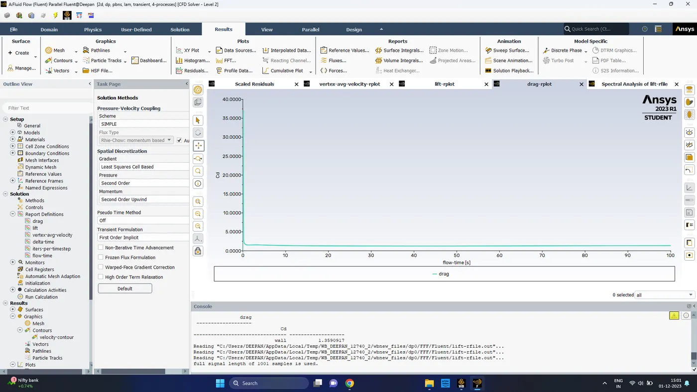
The drag co-efficient obtained is 1.359 whic is very much closer the value mentioned in the paper
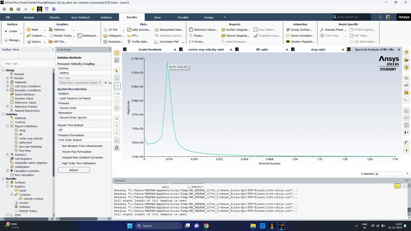
Strouhal No. 1.6
Time: 250s (2500 time steps)
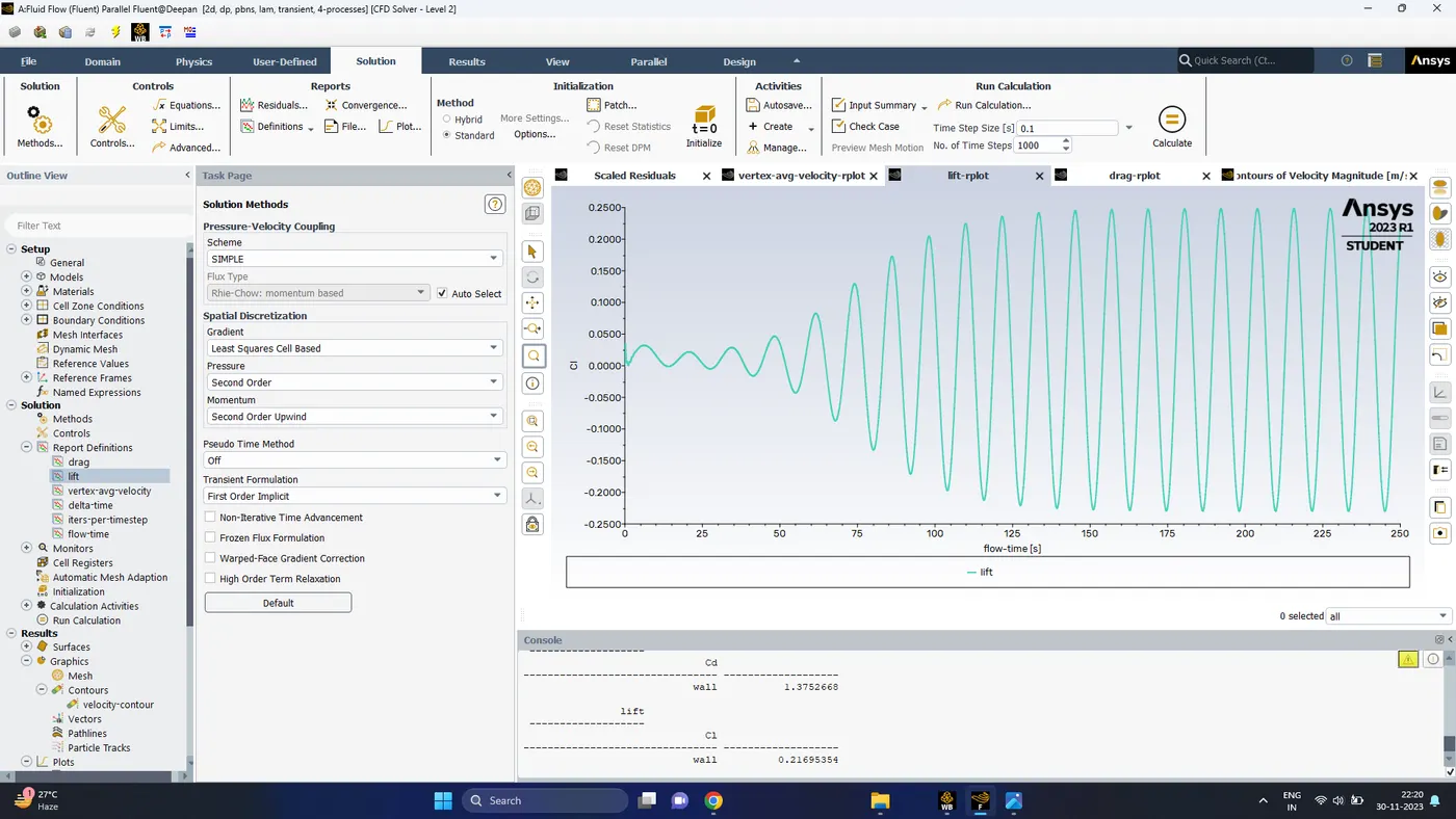
- Lift co-efficient is found to fluctuate with zero reading in mean position to a positive and negative maximum
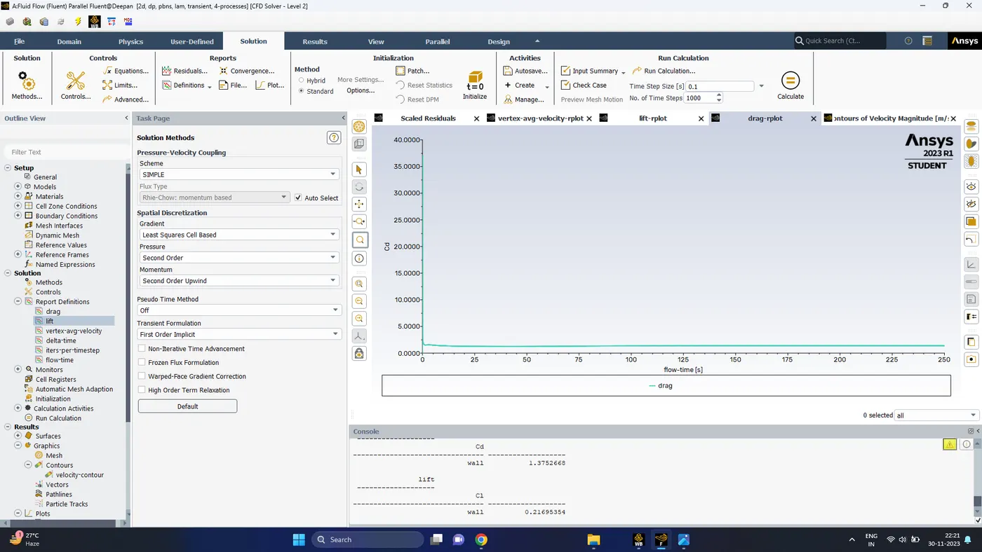
- Co-effiicient of drag is found to have reached a steady state value of 1.375
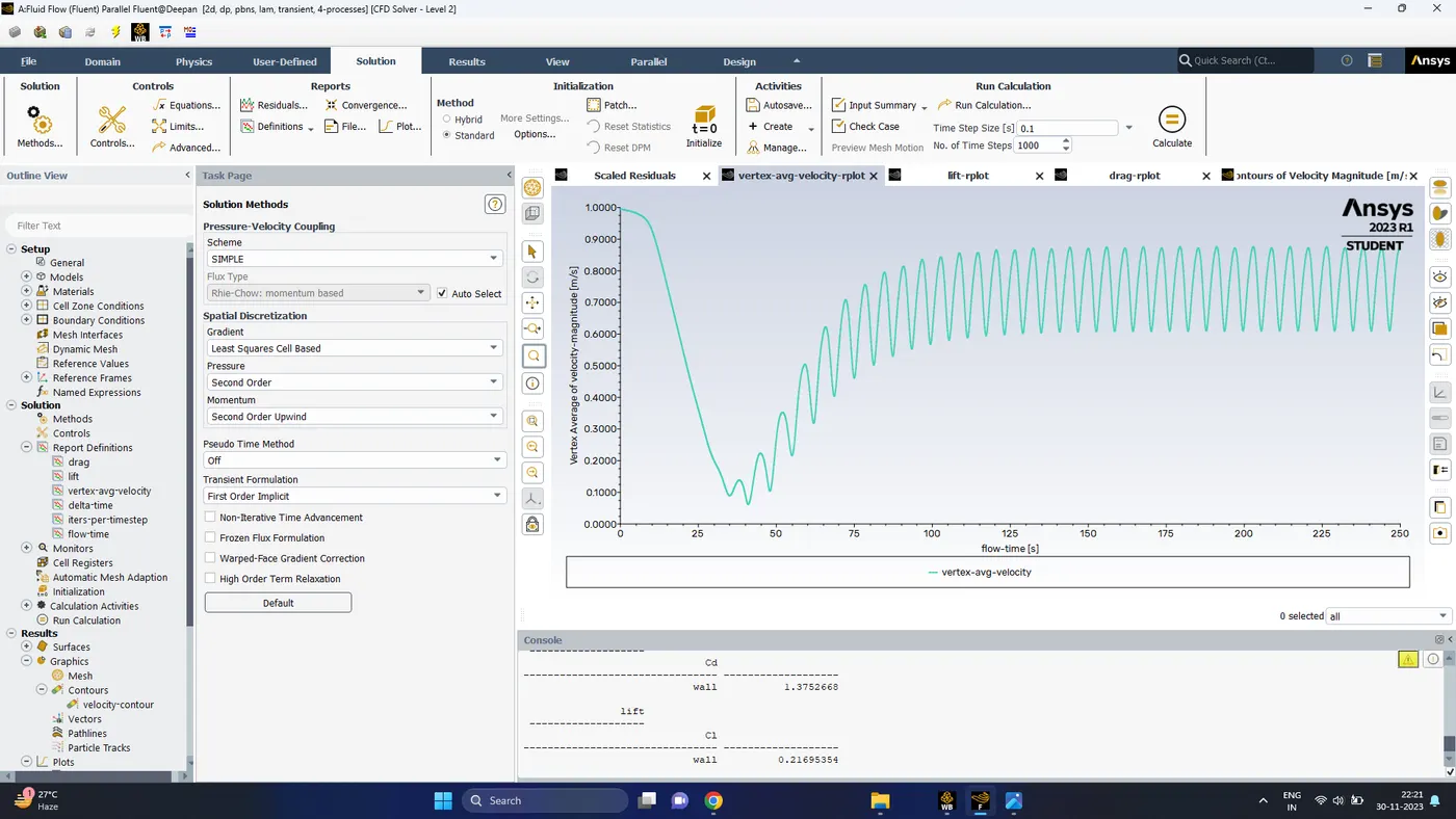
- The monitor point velocity can be seen to have oscillations with a constant repeated fluctuation, which indicates the solution has converged
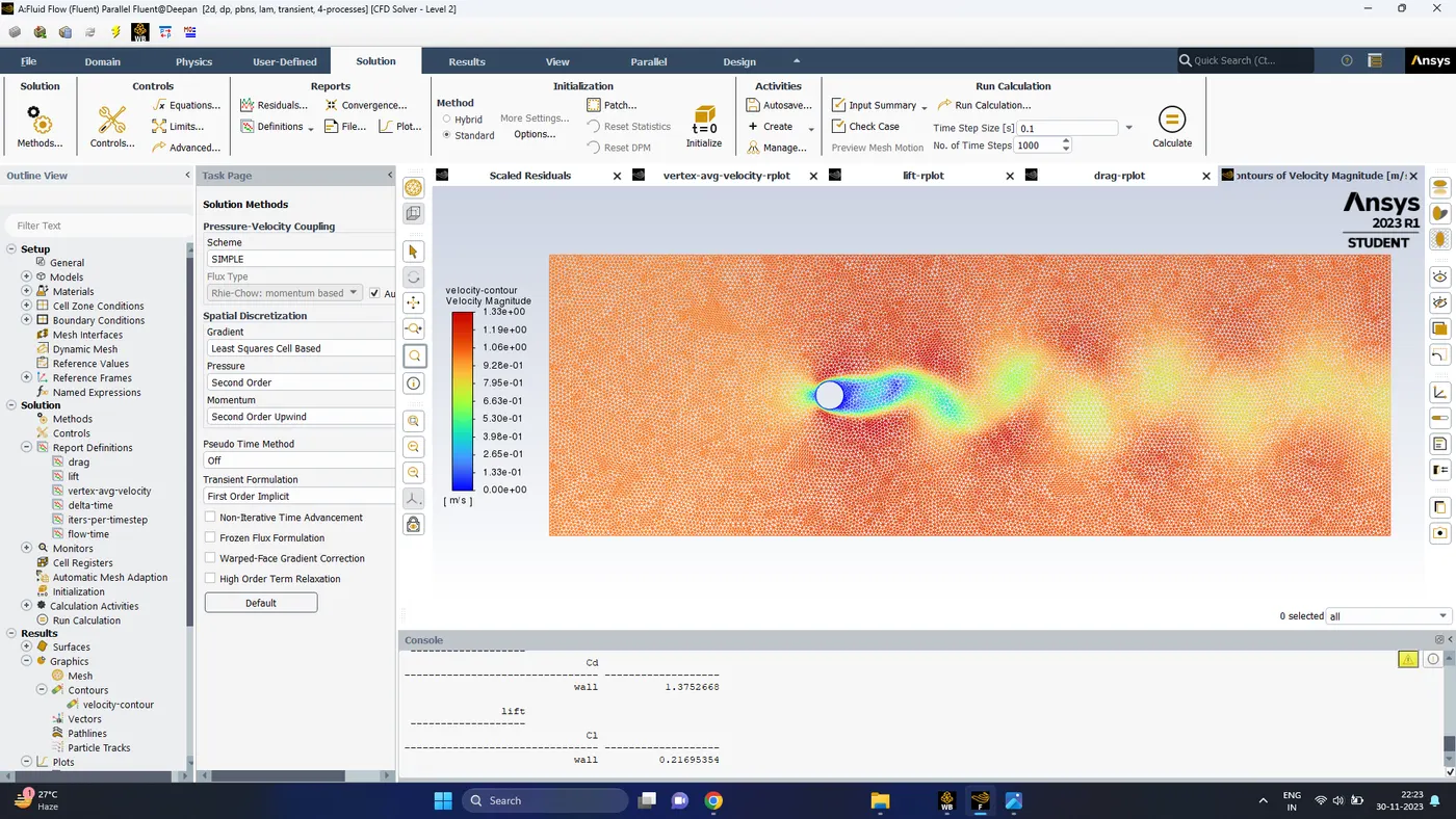
- The contour plot of the flow clearly shows the vortex shedding in downstream of the wall/obstacle
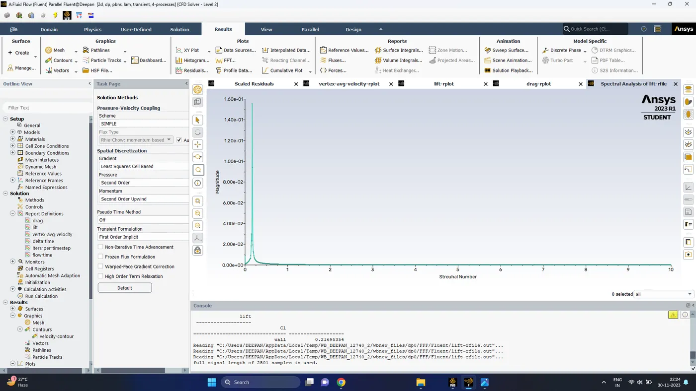
Strouhal number, st = 0.168
| Re=100 | Strouhal Number | Co-efficient of Drag (cd) |
| Steady state | 0.16 | 1.343 |
| Transient 50s | 0.16 | 1.258 |
| Transient 100s | 0.16 | 1.359 |
| Transient State 250s | 0.168 | 1.375 |
| Paper value | 0.157 | 1.335 |
| % Error (Transient 100s) | 1.91% | 1.79% |
| % Error (Transient 250s) | 7.00% | 2.99% |
Results:
- It is observed that the results obtained from steady state analysis differes very much from the actual paper values
- In the transient analysis with 1000 iterations, it is found to have the least error value.
- The value of strouhal number changes marginally when the simulation is continued for higher time steps
- It is observed that the lift co-efficient has an average value of zero, which oscillates from a negative maximum value to a positive maximum
PART B (Steady State Analysis)
1. Reynolds No. 10 (steady state)
Densit, ρ= 1 kg/m`^2`
dynamic viscocity, μ = 0.05 kg/ms
velocity, v = 0.25m/s
1000 iterations
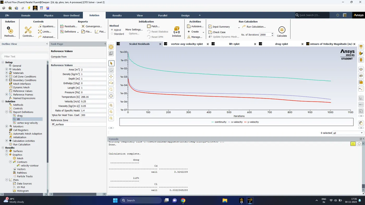
Scaled Residuals
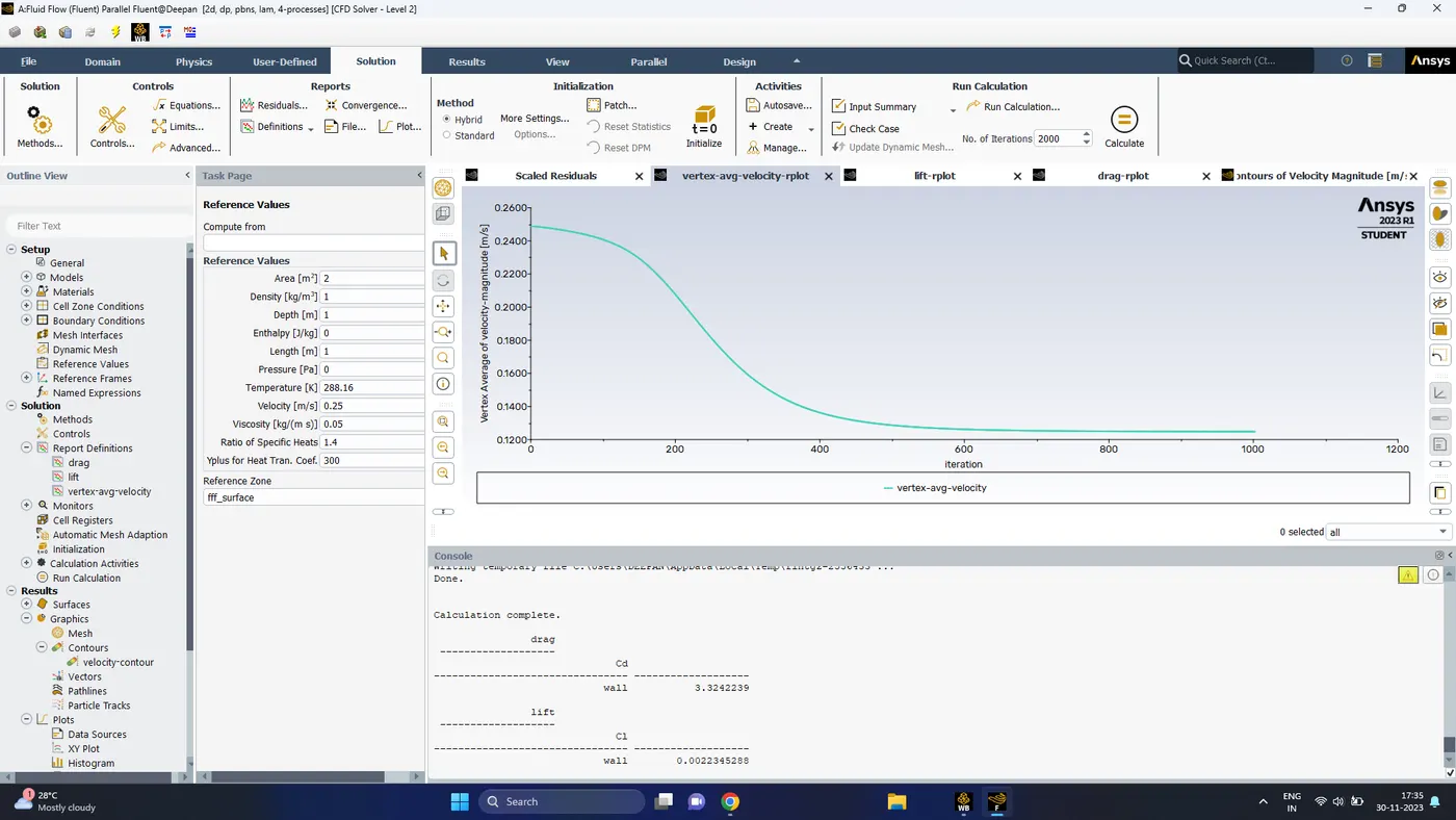
Monitor point velocity
The plot of monitor point velocity shows no sign of vortex shedding and the value has reached a constant value
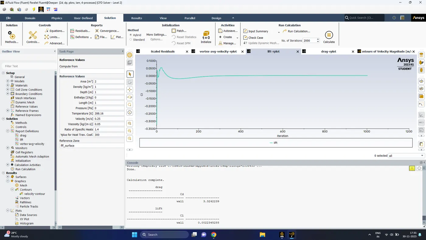
Lift co-efficient (Cl)
The lift co-efficient has attained a constant value of 0.00223, which is very small and hence it does not cause any vortecity in the flow
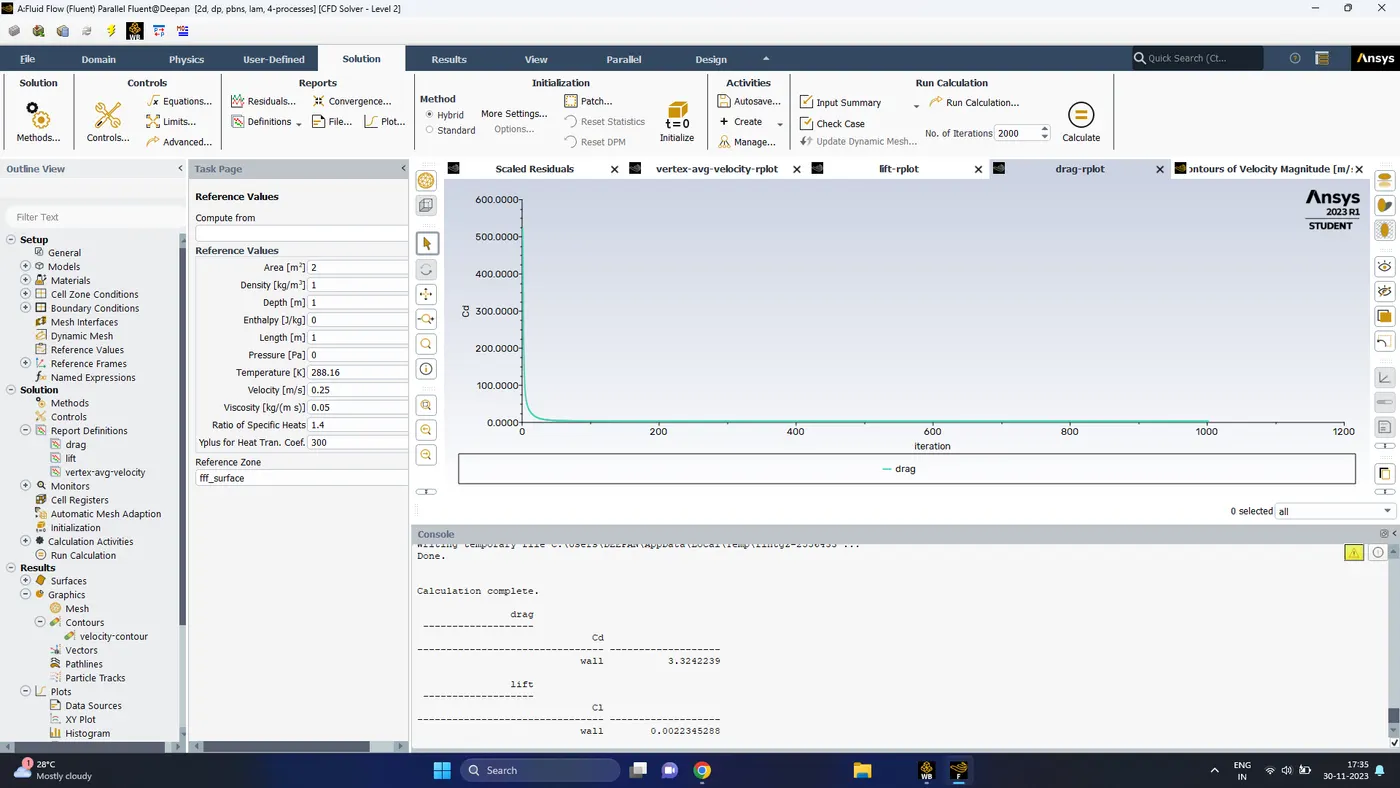
Drag co-efficient (Cd)
Drag co-efficient has attained a contant value of 3.324
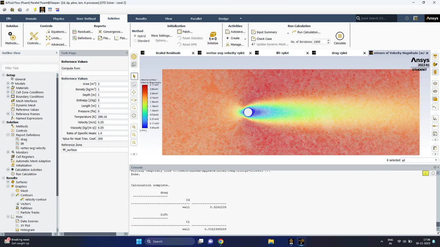
The velocity contur shows the flow simulation with no vortex shedding
2. Reynolds N0. 100 (Steady State)
1000 iterations
Velocity = 2.5 m/s
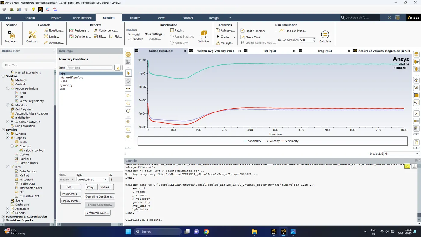
Scaled Residuals
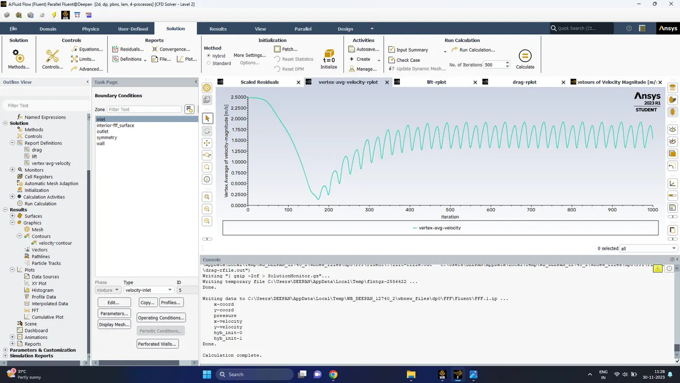
Monitor point velocity
The monitor point velocity shows small fluctuations from its general trend indicating a flow change. It indicates the start of vortex shedding
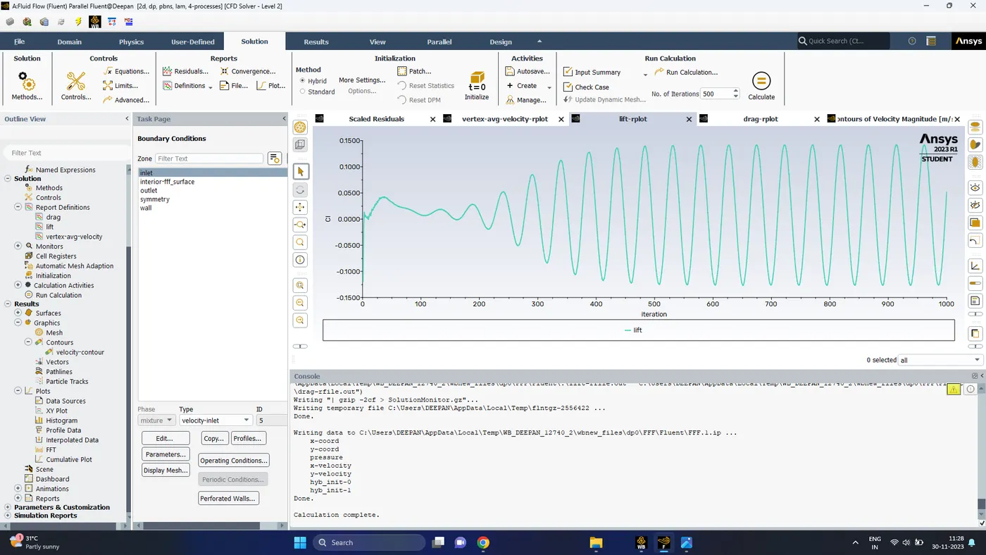
Lift co-efficient
With the reynolds number increased to 100, we dont see a constant value of lift co-efficient, it fluctuates between a negative maximum to positive maximum with zero as mean
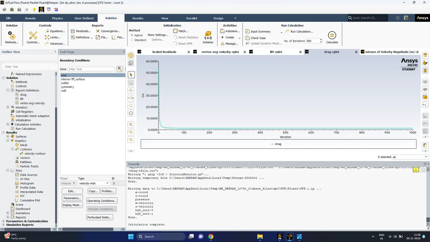
Drag co-efficient
The drag co-efficient has attained a constant value of 1.338
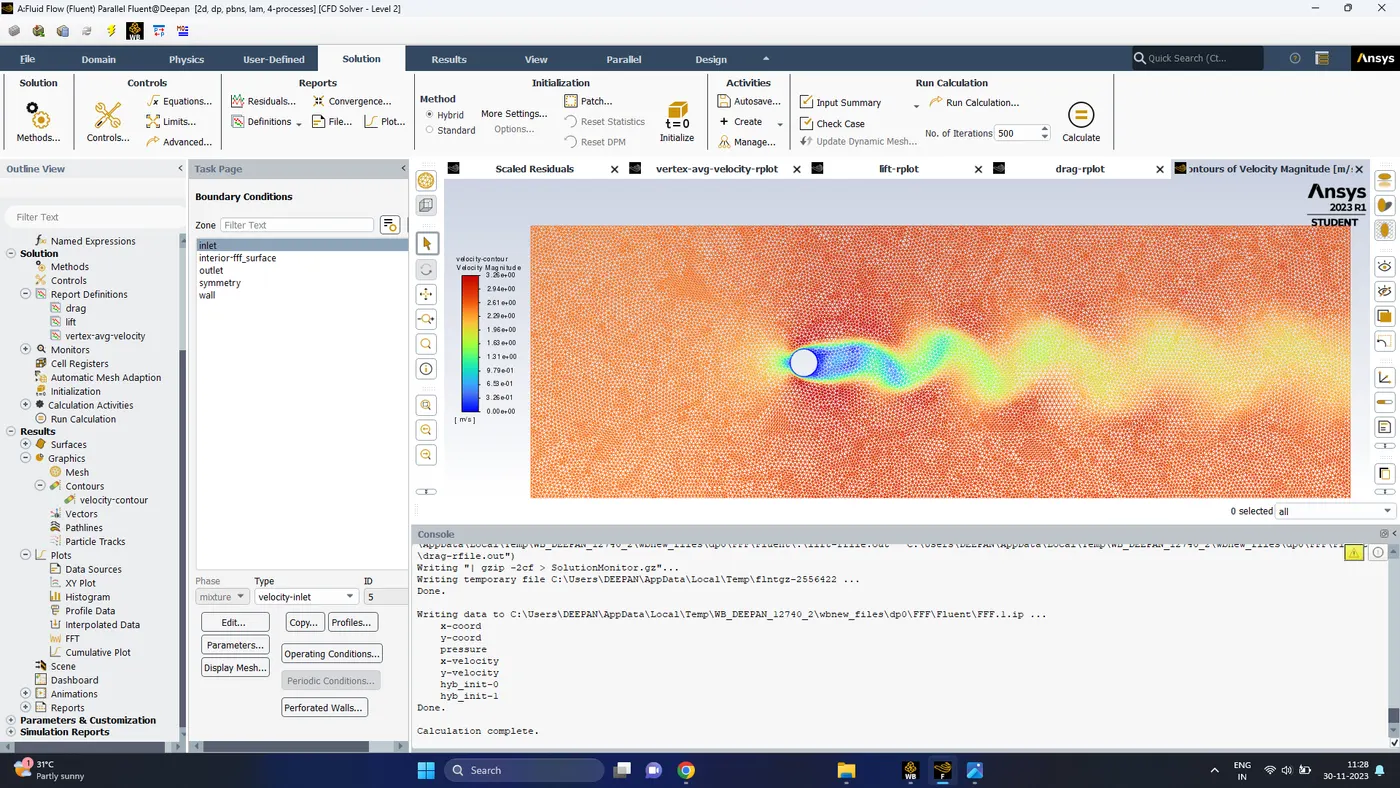
Velocity contour
The velocity contours show a good amount of vortex shedding or eddies in the flow
3. Reynolds number 1000
iterations 750
velocity = 25 m/s
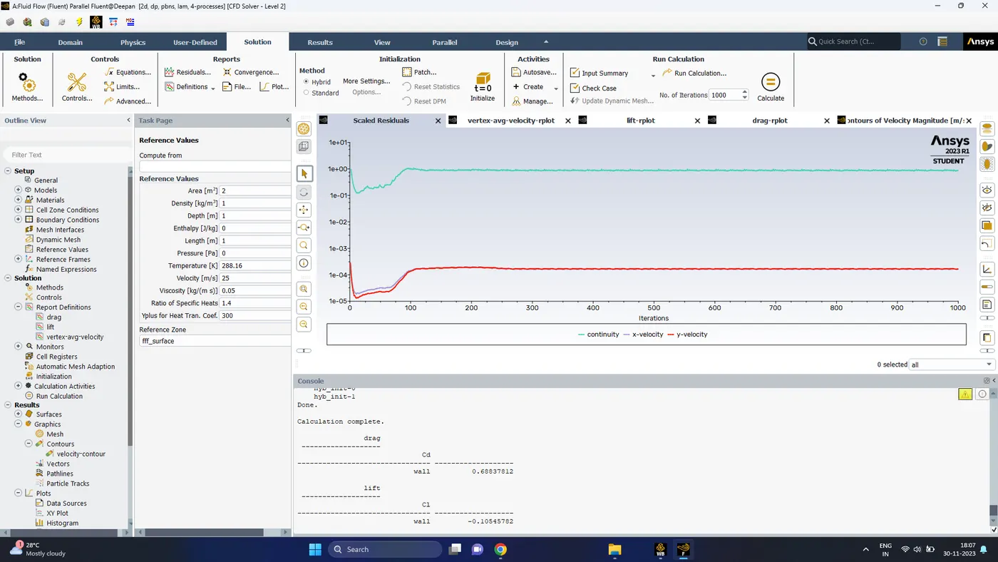
Scaled Residuals
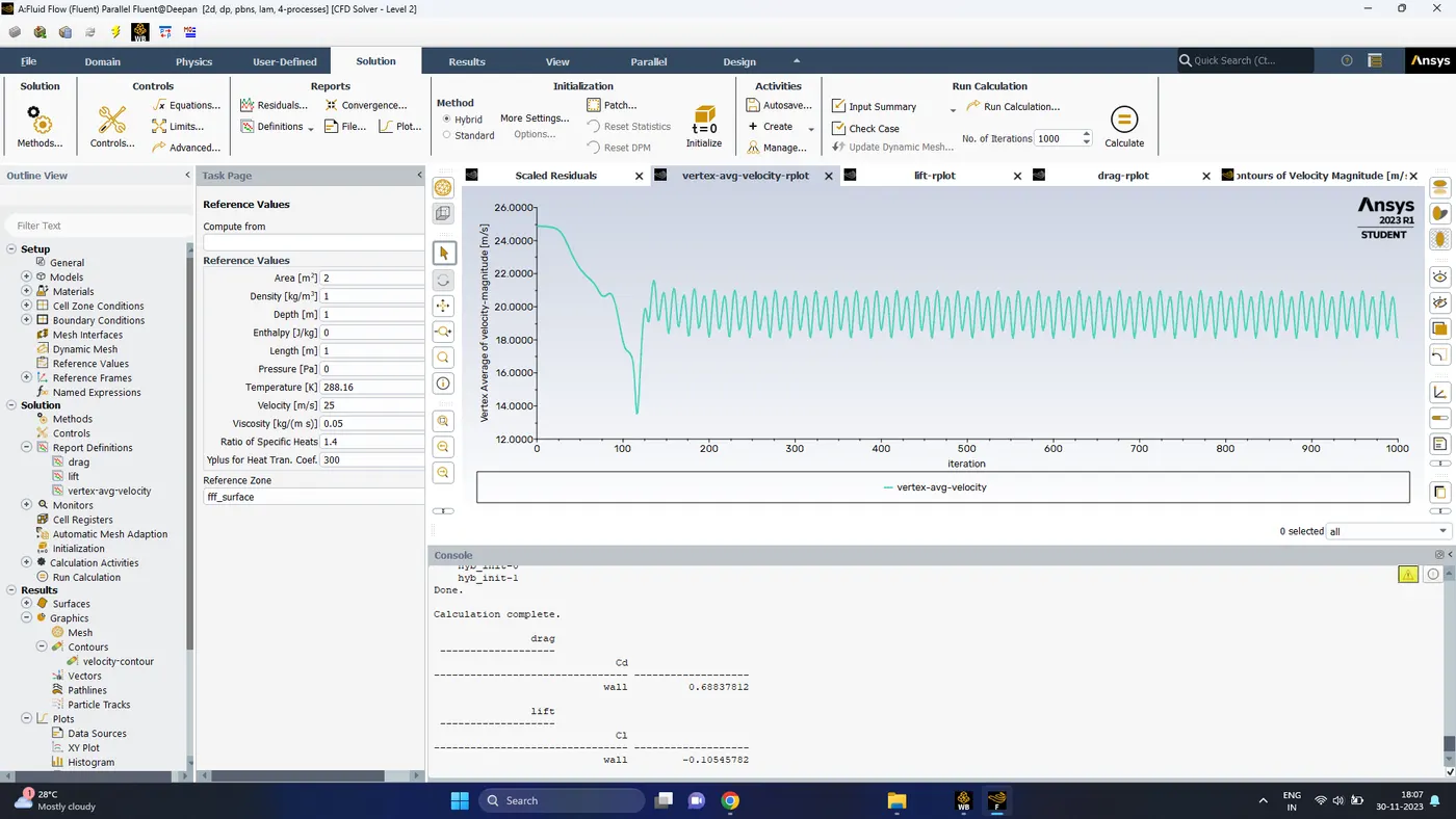
Monitor point velocity
With Reynolds number increased to 1000, we can see a change in monitor point velocity before 100 iterations, it implies the vortex shedding starts much earlier than that occured for reynolds number of 100. This clearly shows in order for vortex shedding to happen, the reynolds number should be sufficiently high
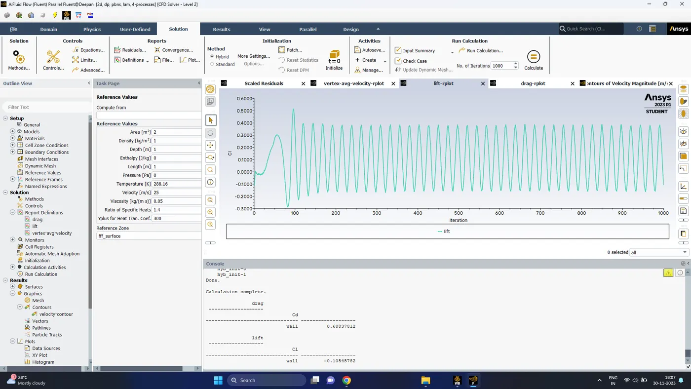
Lift co-efficient
- The lift co-efficient has attained a constant repetitive nature much faster or the flow has converged at a lower iteration number
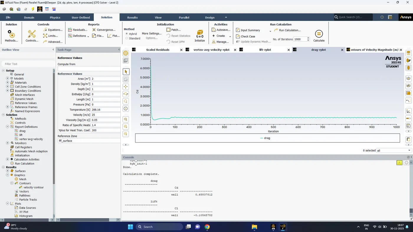
Drag co-efficient
The drag co-efficient starts to show a mild varying pattern with a constant repetitive pattern and it has an approximate value of 0.726
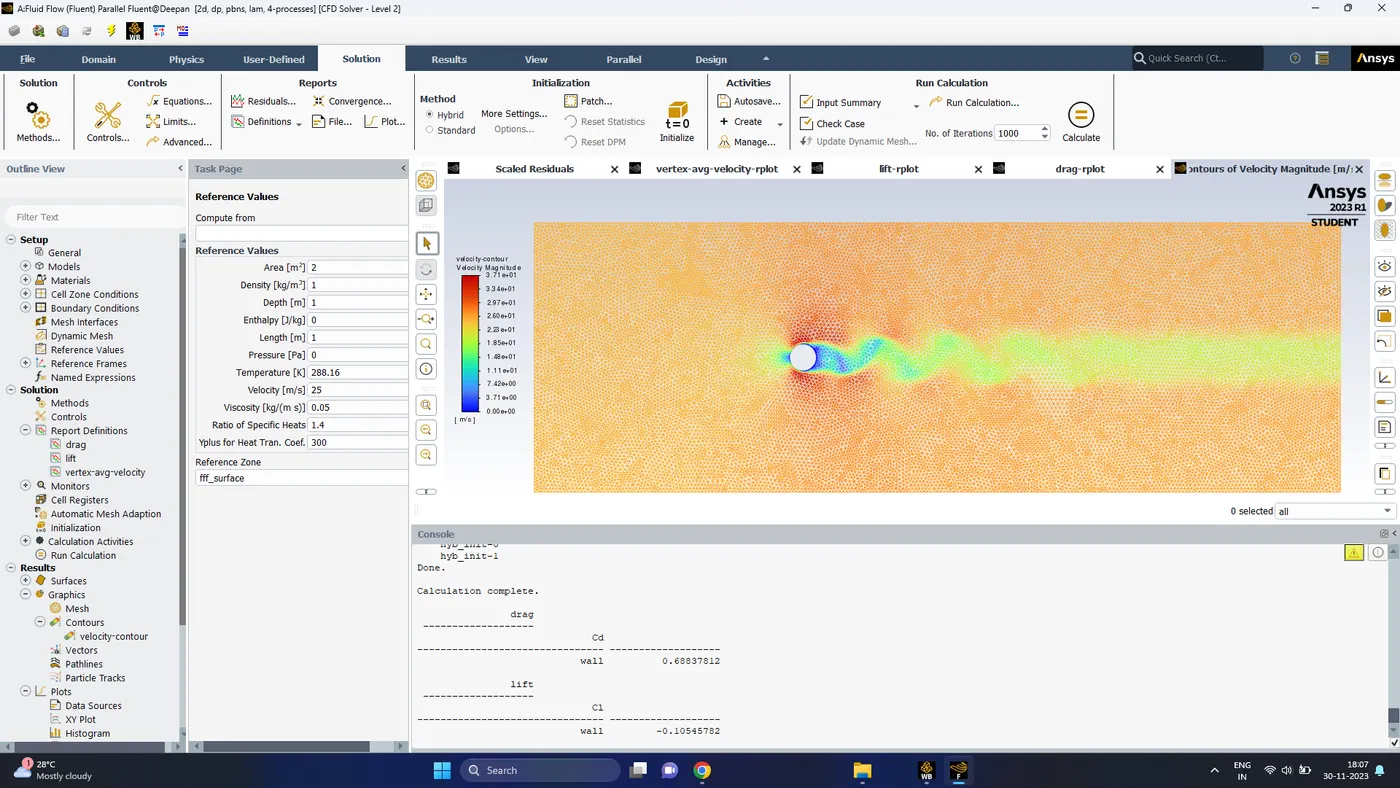
Velocity Contour
4. Reynolds number. 10000
iterations 1000
velocity 250
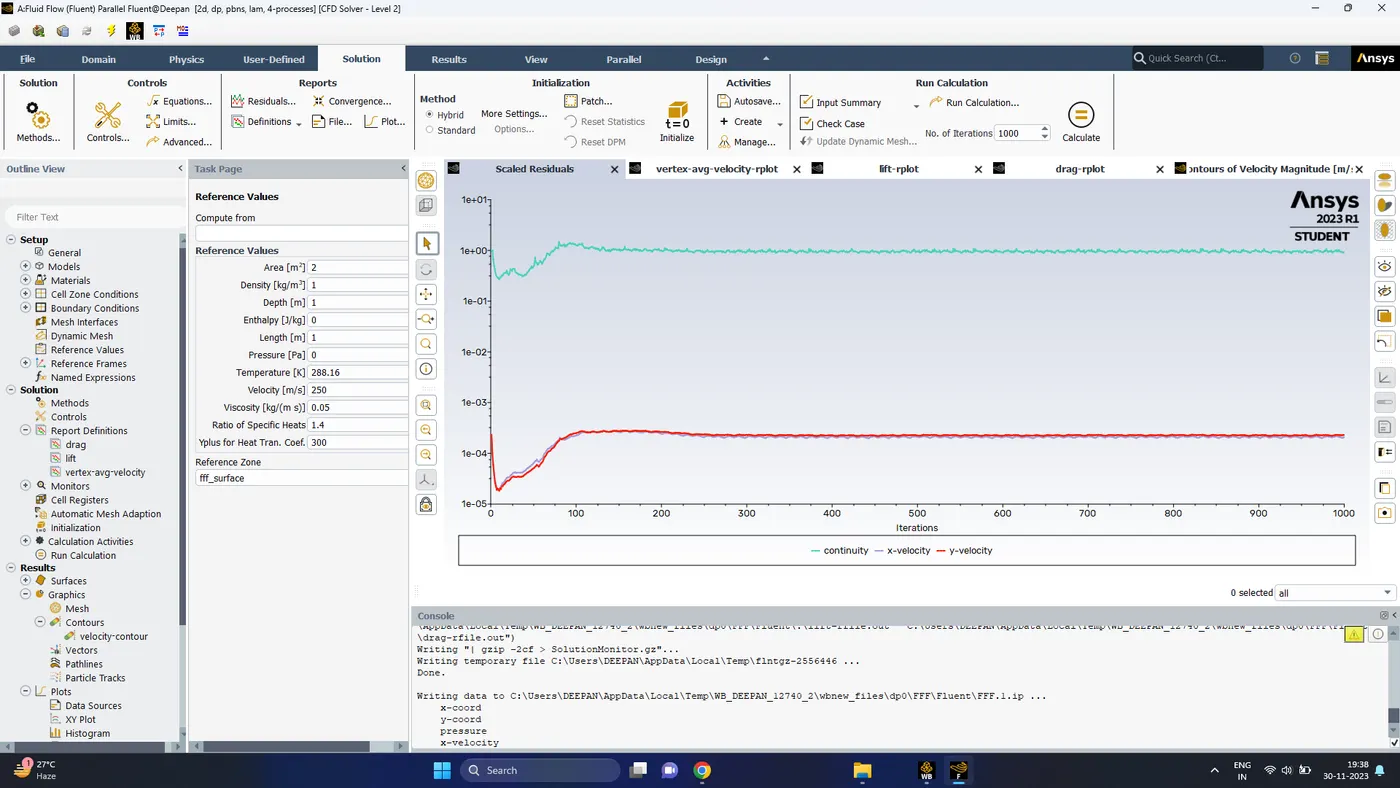
Scaled Residuals
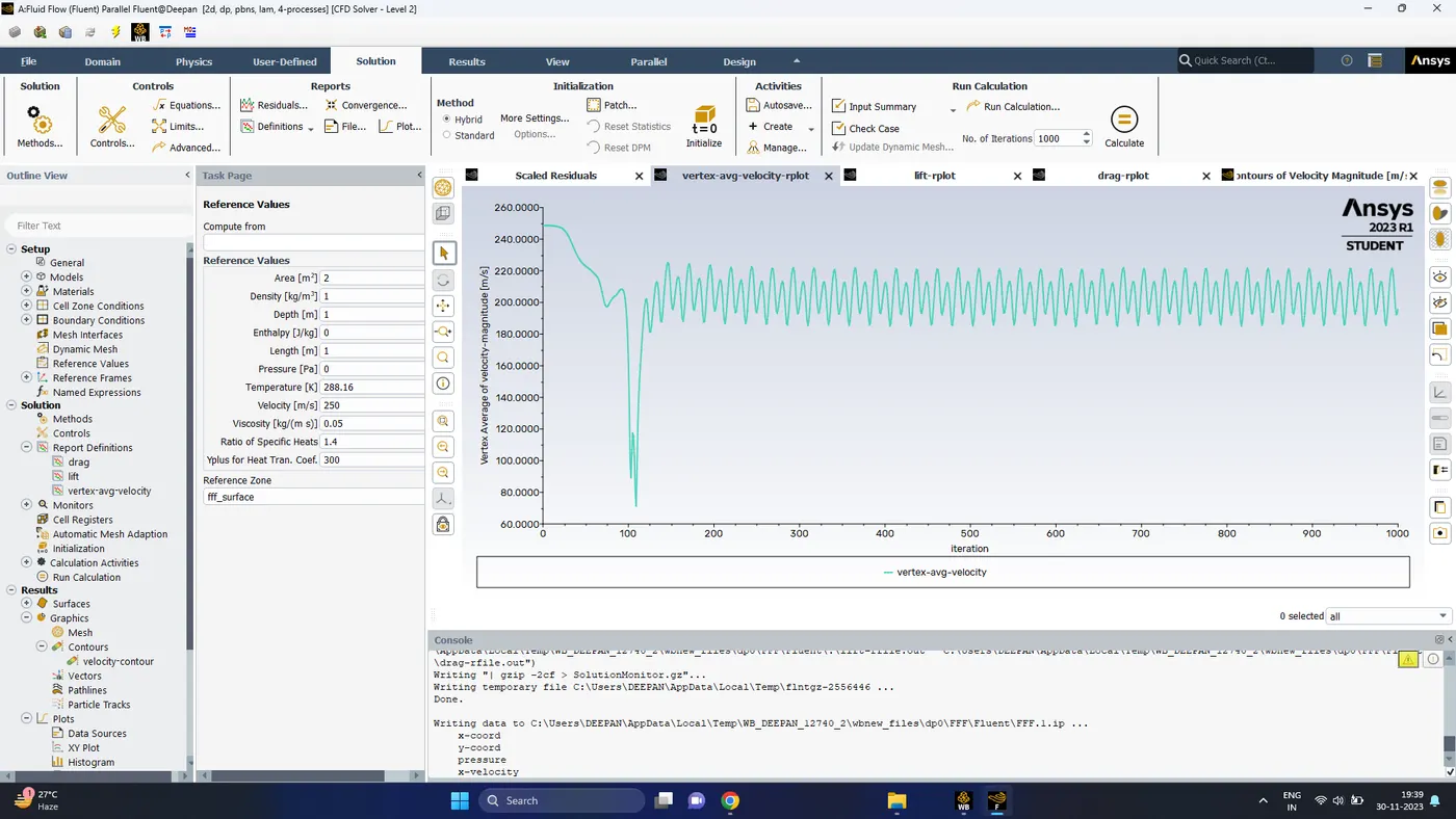
Monitor point velocity
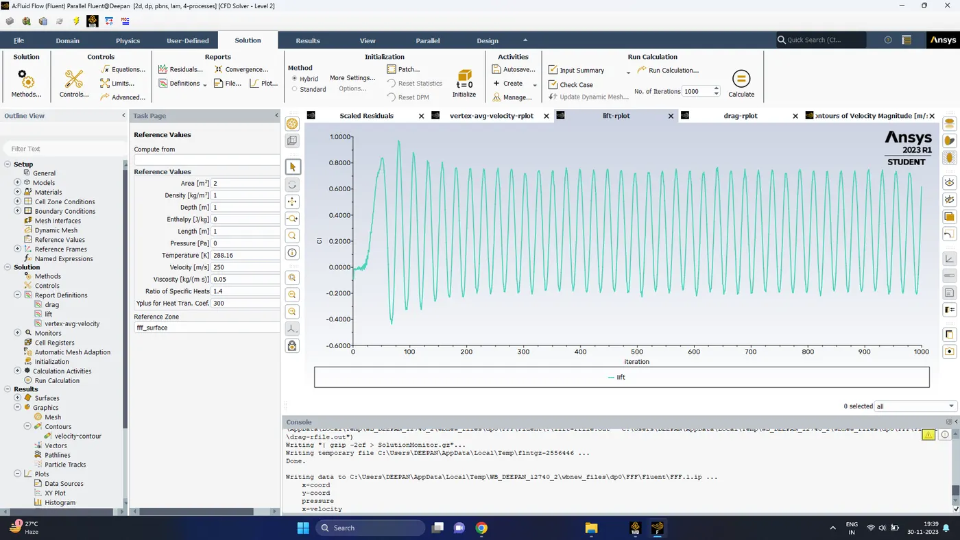
Lift co-efficient
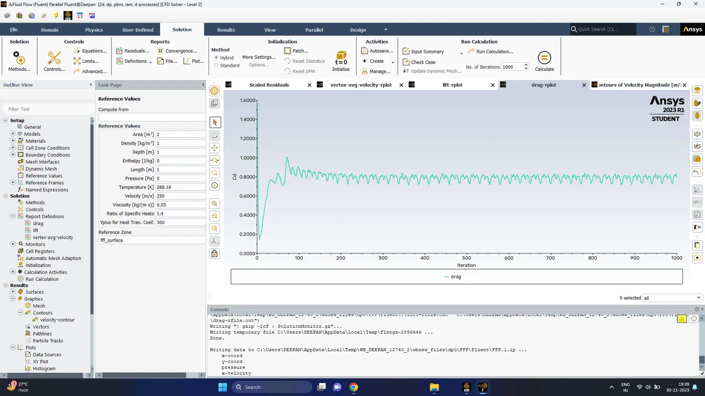
Drag co-efficient
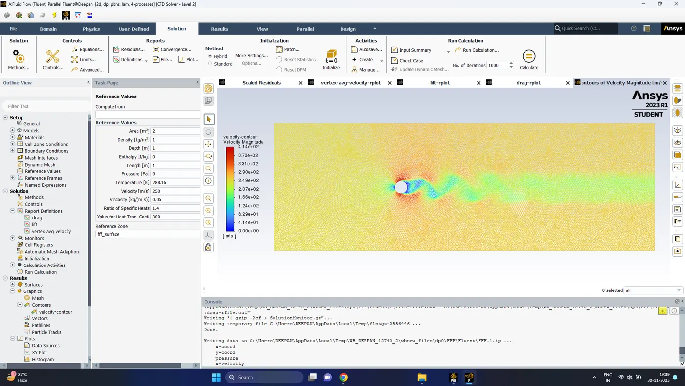
Velocity contour
5. Reynolds number 100000
Iterations 1000
Velocity 2500 m/s
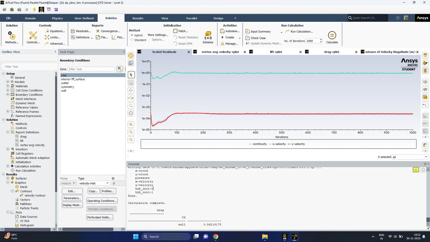
Scaled Residuals
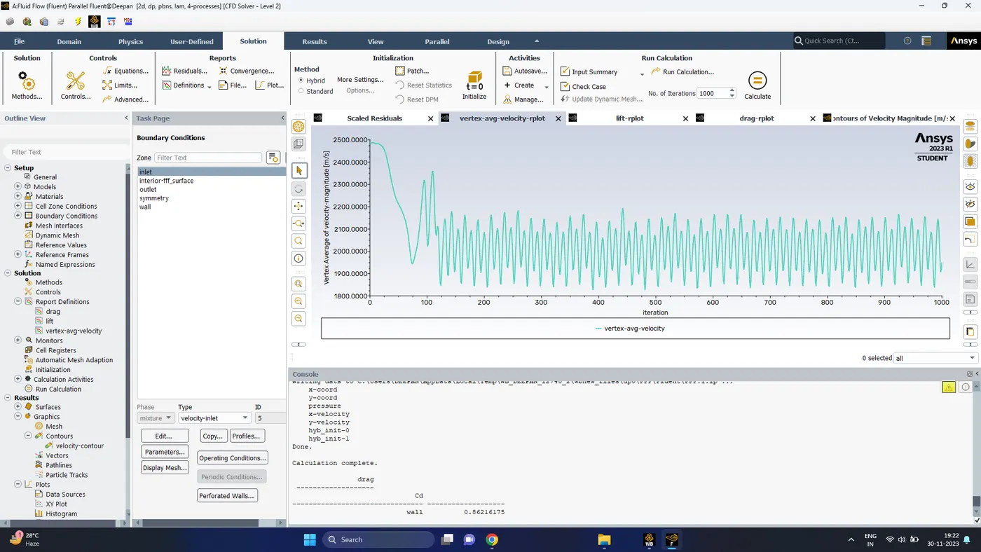
Monitor point velocity
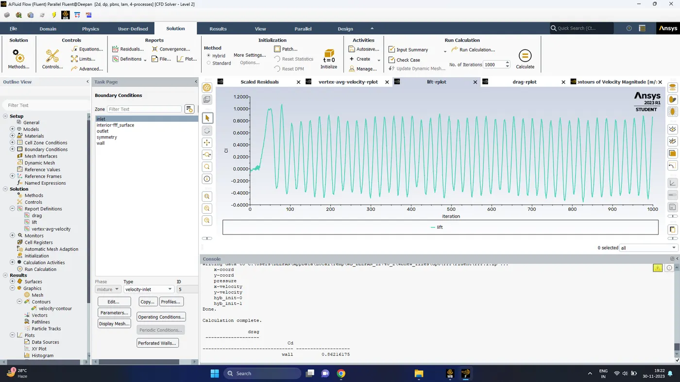
Lift co-efficient
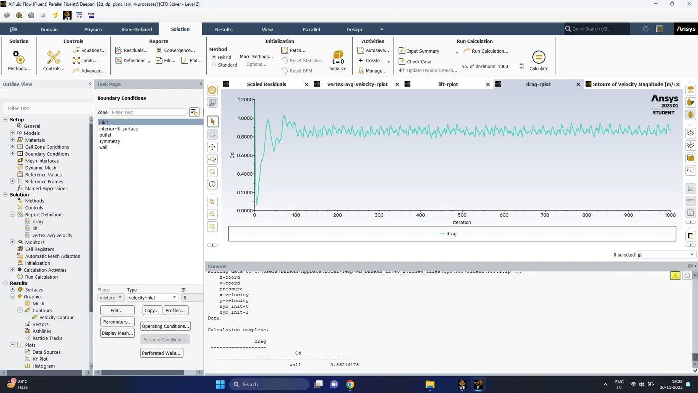
Drag co-efficient
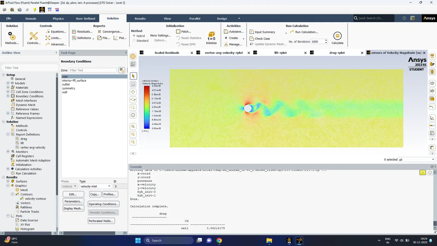
Velocity contour
| Reynolds Number (Re) | Drag co-efficient(Cd) |
| 10 | 3.324 |
| 100 | 1.338 |
| 1000 | 0.726 |
| 10000 | 0.761 |
| 100000 | 0.862 |
Results
- At lower reynolds number, vortex shedding is not visible
- As the reynolds number is increased the vortex shedding is also increased
- The lift co-efficient can be seen at a constant value for reynolds number as no eddies or vortex shedding has occured
- Once the vortes shedding starts the lift co-efficient also fluctuates from a negative maximum to positive maximum
- The drag co-efficient can be seen to decreasewith the reynolds number and reaches a lowest value after that it startes to increase marginally