Week 4.1 - Solving second order ODEs

Aim:

To write a program that solves the following ODE. This ODE represents the equation of motion of a simple pendulum with damping

In the above equation,

g = gravity in m/s2,

L = length of the pendulum in m,

m = mass of the ball in kg,

b=damping coefficient.

Write a program in Matlab\Octave that will simulate the pendulum motion, just like the one shown in the start of this challenge.

use,

L=1 metre,

m=1 kg,

b=0.05.

g=9.81 m/s2.

Simulate the motion between 0-20 sec, for angular displacement=0,angular velocity=3 rad/sec at time t=0.

Errors encountered while coding:

1.

Error:

Code:

Explanation:

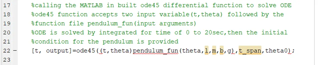
• Ordinary differential equation is solved using ode45 inbuilt Matlab function. There is typo error in the code, while calling the ode45 function '@' needs to be specified before (t,theta)

2.

Error:

Code:

Explanation:

• There is a typo error while writing code, In line no. 34 we plot t and output (2nd column). For calling all elements in row or column matlab we use ':'.
• So instead of ';' rewrite the code as ':'.

3.

Error:

Code:

Explanation:

• In getframe we call for 'get current frame (gcf)' so rewrite the code instead of 'gef' with 'gcf'.

4.

Error:

Code:

Explanation:

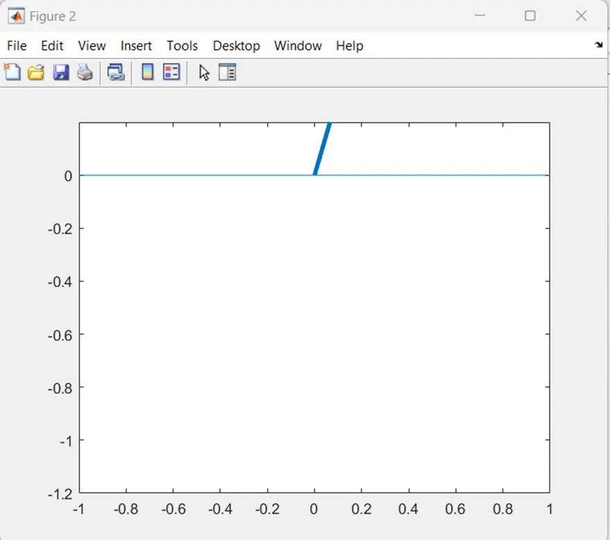
• The output obtained is not desired one, so while checking the code found that in line no. 49 negative sign is missing. Due to which the pendulum is obtained in the 1st & 2nd quadrant.

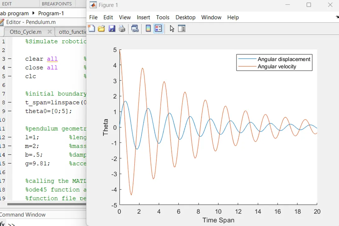
Analysis: By changing various parameters and plotting graph

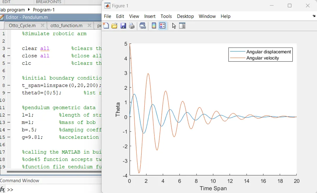
1. v=5 rad/s, l=1m, m=1kg, b=0.5

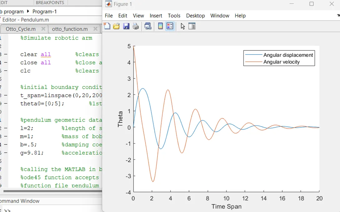
2. v=5 rad/s, l=2m, m=1kg, b=0.5

3. v=5 rad/s, l=1m, m=1kg, b=0.2

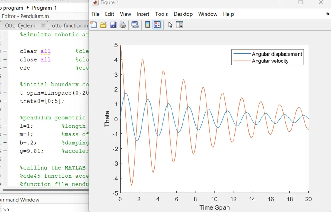
4. v=5 rad/s, l=1m, m=2kg, b=0.5

Matlab Code:

%Simulate robotic arm
 
clear all       %clears the workspace & exceutes the code
close all       %close all the opened windows
clc             %clears the command windows
 
%initial boundary condition
t_span=linspace(0,20,200);      %integrates the ordinary diffferential equation from 0 to 20sec
theta0=[0;3];       %1st row element is initial condition for angular displacement & other is initial condition for angular velocity
 
%pendulum geometric data
l=1;        %length of string
m=1;        %mass of bob
b=.05;       %damping coefficient
g=9.81;     %acceleration due to gravity
 
%calling the MATLAB in built ode45 differential function to solve ODE
%ode45 function accepts two input variable(t,theta) followed by the
%function file pendulum_fun(input arguments)
%ODE is solved by integrated for time of 0 to 20sec,then the initial
%condition for the pendulum is provided
[t, output]=ode45(@(t,theta)pendulum_fun(theta,l,m,b,g),t_span,theta0); 
 
%output array is column vector of time point 't' and a solution array
%'output'
%each row in 'output' corresponds to a time returned in the corresponding row
%of 't'
 
 
%plotting angular velocity and displacement vs time 
figure(1)       %plotting window 1
hold on         %hold on all the values till the plotting is complete
plot(t,output(:,1))     %plot time vs all rows of 1st column of 'output' array i.e. angular displacement
plot(t,output(:,2))     %plot time vs all rows of 2nd column of 'output' array i.e. angular velocity
xlabel('Time Span')     %provide x label to the plot
ylabel('Theta')         %provide y label to the plot
legend('Angular displacement','Angular velocity')       %provide legend to the plot
 
 
%create animation for pendulum motion
ct=1;       %counter variable
for i=1:length(t)       %for loop
    x0=0;       %pendulum tied to the fixed, x coordinate
    y0=0;       %pendulum tied to the fixed, y coordinate
    
    %x1 & y1 value change w.r.t looping iteration
    %negative sign is mentioned 
    x1=-1*sin(output(i,1));     %bob tied to the string, x coordinate
    y1=-1*cos(output(i,1));     %bob tied to the string, y coordinate
    
    %plotting the position of pendulum
    figure(2)       %plotting window 2
    plot([x0,x1],[y0,y1],'linewidth',3)     %plot string from (x0,y0) to (x1,y1)
    hold on        %hold on all the values till the plotting is complete  
    line([-1 1],[0 0])      %plot the line to which the pendulum is fixed 
    plot(x1,y1,'.','Markersize',100,'color','r')         %plot the marker of size 50 which represent bob 
    hold off       %hold is put off
    axis([-1 1 -1.2 0.2])           %fix the plotting window axis
    
    %using getframe function to capture the current plotting frame
    M(ct)=getframe(gcf);        %each captured frame is stored in the 'M' array
    ct=ct+1;            %counter variable is increased
end       %end of for loop
 
 
%creating movie file using the captured frame array
videofile=VideoWriter('Pendulum_motion.avi');      %creates videowriter object to write video data to an AVI file
open(videofile)         %open file for writing video data
writeVideo(videofile,M)         %write video data to file
close(videofile)        %close file after writing video data

Function Code:

% function code
% output solution data is obtained from the fuction
%function is called along with input arguments
 
function [dtheta_dot]=pendulum_fun(theta,l,m,b,g)
theta1=theta(1);
theta2=theta(2);
 
dtheta1_dot=theta2;         %equation 1
dtheta2_dot=-(b/m)*theta2-(g/l)*sin(theta1);        %equation 2
 
dtheta_dot=[dtheta1_dot;dtheta2_dot];       %output array consist of 1st column angular displacement, 2nd column angular velocity
 
end     %end of function 

Output:

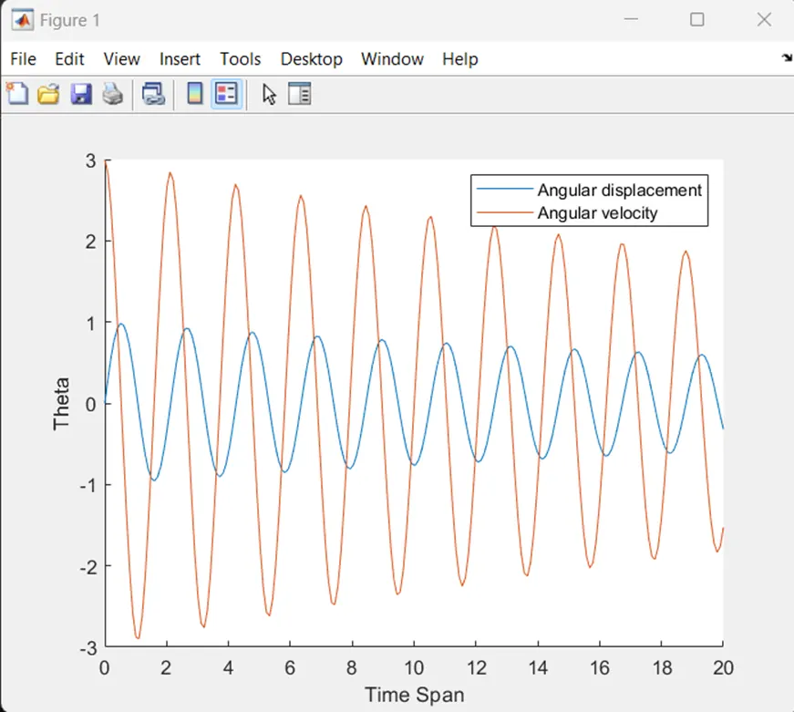
• Plotting angular displacement, angular velocity Vs Time for the given data. Further, animation video file is created.

Animation File:

https://drive.google.com/file/d/1PmQkmiwG_AVAAi4mGO43JuTJvPFmP1PI/view?usp=sharing