Week 4.1 - Solving second order ODEs
Solving Second order ODEs
Aim:
To develop a MATLAB program that simulates and animates the motion of a pendulum, using the principles of second-order differential equations (ODEs), in order to visually demonstrate the dynamic behavior of a pendulum and enhance comprehension of its complex motion.
Introduction:
The simulation and animation of a pendulum’s motion is a compelling application of a physics and computational techniques. Pendulums are ubiquitous in nature and engineering, and their behavior can be described by second-order ordinary differential equations (ODEs) by creating a MATLAB program to model a pendulum’s dynamics and visualize its motion, we can gain a deeper insight into the fundamental principles of harmonic motion and oscillatory systems.
In this project, we aim to develop a program that accurately represents the motion of a simple pendulum, taking into account factors such as the pendulum length and initial conditions. By solving the governing ODEs numerically, we can calculate the pendulum position as a function of time. The resulting data is then used to create a dynamic animation that illustrates the pendulum’s oscillatory behavior.
It provides a tangible, visual representation of the concepts of periodic motion and energy conservation, offering a hands-on approach to understanding complex physics.
Explanation:
We are setting out to understand and visualize the motion of a pendulum. A pendulum is like what you might see on a pendulum clock, where the weight swings back and forth. But, to really understand how it moves and why it swings, we need some help from math and computers.
1. Simulating Pendulum Motion:
· To start, we want to use a computer program like MATLAB to simulate the motion of a pendulum. This means we’ll use the computer to mimic what real pendulum would do if we set it in motion.
2. Pendulum Details:
· Pendulums come in different shapes and sizes. Some have long strings, and some have short ones. The length of the string or rod and how we push it when starts swinging all affect how it moves. So, we need to consider these details when we create our simulation.
3. Math Behind the Pendulum:
· Pendulums follow some rules that can be described using math. We’re going to use the mathematical rules to tell the computer how the pendulum should move. The main rule is called “Second-order ordinary differential equation” (ODE), which sounds complicated, but it’s just a way to describe how the pendulum swings.
4. Solving the Math:
· We’ll use the computer to solve these mathematical rules and figure out where the pendulum will be at different moments in time. This way, we can create a kind of “map” that shows the pendulum’s position as it swings back and forth.
5. Creating an Animation:
· With this map of positions, we can create an animation. Think of it like of how that shows each moment in time. This animation will give us a clear picture of how the pendulum moves, and we can watch it swing on the computer screen.
Solved Errors
Error 1 :

Line No. 15
Line with Error: theta_0 = (0,3);
Correction: theta_0 = [0;3];
I replaced the parenthesis with square brackets. This is necessary to define theta_0 as an array or vector with the elements 0 and 3.
Error 2:
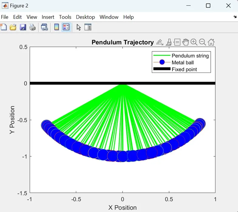
Correction:
Line No. 57
Line with Error : Made mistake in usage of hold on and hold off commands.
Correction : Insert a hold off option to avoid overlagging of the pendulum.
Error 3:
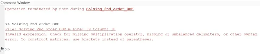
Line No. 39 to 44:
Code with error:
x1(i)0 = 0;
y1(i)0 = 0;
% Varied value for end point of pendulum
x1(i) = l*sin(results(i,1));
y1(i) = -l*cos(results(i,1));
· In the error code, attempted to create a variable named x1(i) = 0 and y1(i) =0. Variable names cannot contain parenthesis and numbers without valid variable naming conventions.
Correction:
x0 = 0;
y0 = 0;
% Varied value for end point of pendulum
x1 = l*sin(results(i,1));
y1 = -l*cos(results(i,1));
· In the corrected code, the error was fixed by using variable names x0 and y0. The MATLAB naming conventions, x0 and y0 are set to 0, indicating that the initial coordinates of the pendulum’s endpoint are both at the orgin (0,0).
Error 4:
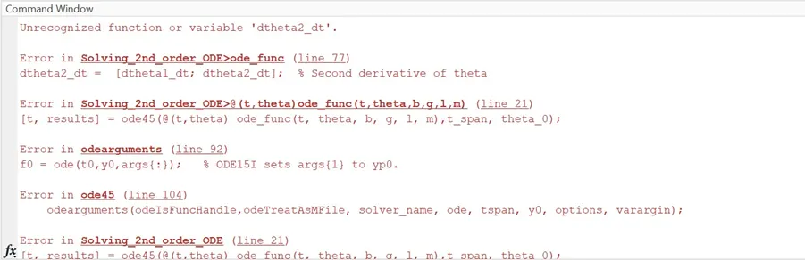
Line No. 74 to 78:
Code with error:
theta1 = theta(1);
theta2 = theta(2);
dtheta1_dt = -(b/m)*theta2 - (g/l)*sin(theta1);
dtheta2_dt = [dtheta1_dt; dtheta2_dt];
dtheta_dt = theta2;
Correction:
theta1 = theta(1);
theta2 = theta(2);
dtheta1_dt = theta2;
dtheta2_dt = -(b/m)*theta2 - (g/l)*sin(theta1);
dtheta_dt = [dtheta1_dt; dtheta2_dt];
Error 5:
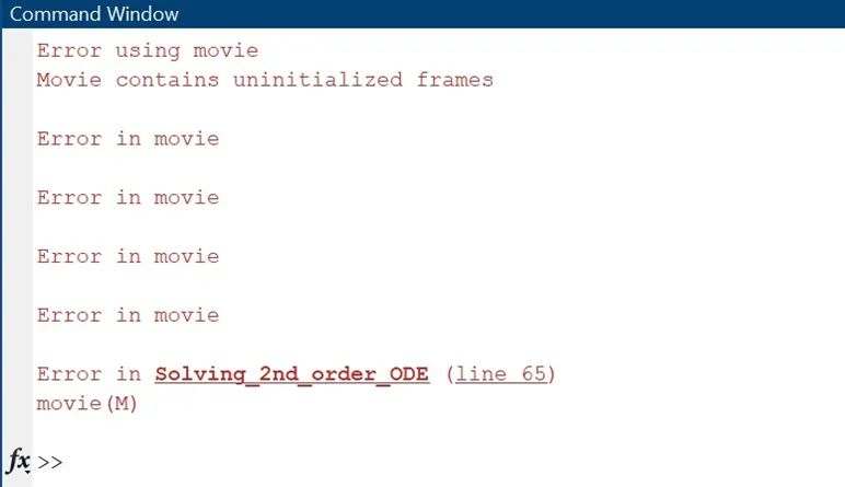
Line No. 65:
Code with error: M(i) = getframe(gcf);
( Must be replaced in inside the forloop)
· In this line we can see the error in movie while creating a animation, and we cannot able to capture the frame because of the code is we provided after the end of the for loop so that we can get a error in movie. For that we need to write this code inside the for loop before the end command.
Code with comments
% Solving Second order ODEs
clear all
close all
clc
% Inputs
l = 1; % length of the pendulum(m)
m = 1; % Mass of the pendulum(kg)
b = 0.05; % Dampind coefficient
g = 9.81; % Gravity in m/s2
% Initial Condition
theta_0 = [0;3]; % Initial angle in radians
% time points
t_span = linspace(0,20,500); % Create a time span from 0 to 20 sec with 500
% Solve ODE
[t, results] = ode45(@(t,theta) ode_func(t, theta, b, g, l, m),t_span, theta_0);
% Solve the ODEs using ode45 with the specified function ode_45, and initial conditions theta_0
% Plot the pendulum angles as a function of time
figure(1) % Create a new figure with the number 1
plot(t,results(:,1), 'r', 'linewidth', 1.5); % Plot the first column of results (theta1) in red
hold on % Hold the current plot for overlay
plot (t,results(:,2), 'b', 'Linewidth',1.5); % Plot the first column of results (theta1) in blue
xlabel('Time (s)') % Label for the x-axis
ylabel('Angle (radians)') % Label for the y-axis
legend('theta_1', 'theta_2') % Add a legend to distuinguish the two curves
title('Pendulum Motion') % Title of the plot
for i = 1:length(t)
% Origin or starting position of pendulum which is fixed
x0 = 0;
y0 = 0;
% Varied value for end point of pendulum
x1 = l*sin(results(i,1)); % X-coordinate for the pendulum end
y1 = -l*cos(results(i,1)); % Y-coordinate for the pendulum end
figure(2) % Create a new figure with the number 2
plot([x0 x1], [y0 y1],'g', 'LineWidth',1.5); % Plot the pendulum string in green
hold on
plot(x1,y1,'Marker','o','MarkerSize',20,'MarkerFaceColor','b') % Plot the metal ball at the end
xlabel('X Position')
ylabel('Y Position')
title('Pendulum Trajectory')
plot([-1 1 ],[0,0],'color','black','LineWidth',5)% Plot a horizontal line for the fixed point
axis([-1 1 -1.5 0.5 ]) % Set the axis limits
legend('Pendulum string', 'Metal ball','Fixed point'); % Add a legend
pause(0.01) % Pause for a short time to create the animation effect
hold off % Release the current plot
M(i) = getframe(gcf); % Capture the current figure as a frame
end
% Create a movie file
movie(M)
videofile = VideoWriter('Sec_Order_ODE', 'Uncompressed AVI'); % Create a video file
open(videofile) % Open the video file
writeVideo(videofile,M) % Write the frame to the video file
close(videofile) % Close the video file
% Plot the results
function dtheta_dt = ode_func(t ,theta,b,g,l,m)
theta1 = theta(1); % Extract the first angle from the input
theta2 = theta(2); % Extract the second angle from the input
dtheta1_dt = theta2; % First derivative of theta1
dtheta2_dt = -(b/m)*theta2 - (g/l)*sin(theta1); % Second derivative of theta
dtheta_dt = [dtheta1_dt; dtheta2_dt]; % Combine the derivative into a column vector
end
Explanation of Code:
theta_0 = [0;3];
· theta_0 is a variable that is being defined or initialized and [0;3]; is an array enclosed in square brackets. 0 is the initial angle (in radians) and 3 is the initial angular velocity (how fast the pendulum is moving at the start).
t_span = linspace(0,20,500);
· t_span is a variable that is being defined or initialized.
· Linspace is a function is used to create an array of equally spaced values between the two specified end points.
· The first argument 0 is the starting point of the time span.
· The second argument 20 is the ending point of the time span.
· The third argument 500 is the number of equally spaced points or values you want within the time span.
[t, results] = ode45(@(t,theta) ode_func(t, theta, b, g, l, m),t_span, theta_0);
· [t, results] is way to define two variables at once. t and results will store the points and the the corresponding results of the simulation.
· ode45 function used for solving ODEs numerically. It uses an adaptive time-stepping method to approximate the solution.
· @(t,theta) ode_func(t, theta, b, g, l, m is a function that represents the ODEs to be solved. The variables ‘t’ and ‘theta’ represents the time and the state of the system (angles and angular velocities).
· ode_func is the function that calculates the derivatives of theta.
· b, g, l, m are based on these variables and the systems parameters.
figure(1)
plot(t,results(:,1), 'r', 'linewidth', 1.5);
hold on
plot (t,results(:,2), 'b', 'Linewidth',1.5);
xlabel('Time (s)')
ylabel('Angle (radians)')
legend('theta_1', 'theta_2')
title('Pendulum Motion')
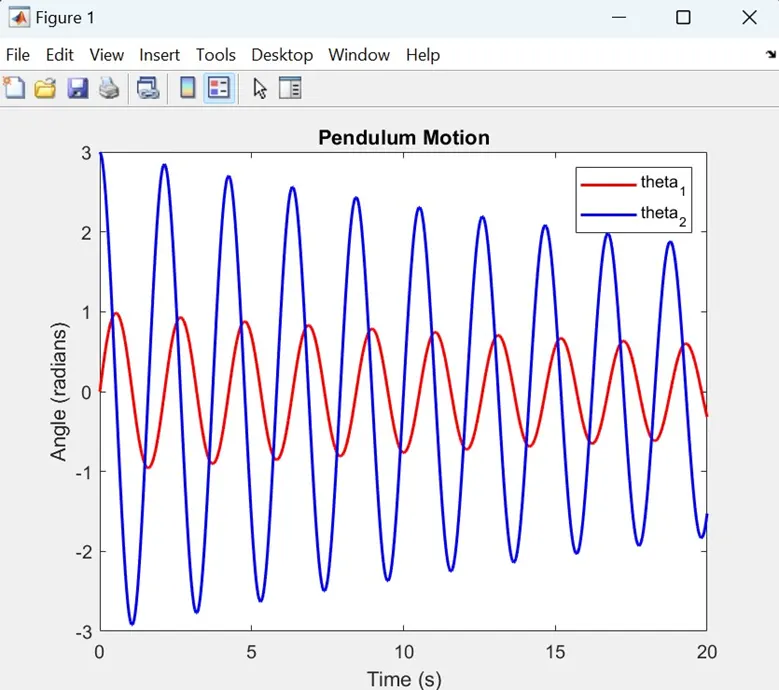
· plot(t,results(:,1), 'r', 'linewidth', 1.5); This line of code creates a plot, it values from the ‘t’ variable on the x-axis (representing time) and the first column of the results matrix on the y-axis. linewidth, 1.5 makes the line thicker.
· plot (t,results(:,2), 'b', 'Linewidth',1.5); This line creates a second plot on the same figure just like in the previous line. Only difference the colour variant has “blue” for the metal ball ion the simple pendulum.
· xlabel('Time (s)') This commands adds a label to the x-axis. It represents time in seconds.
· ylabel('Angle (radians)') This command adds a label to the y-axis. It represents the angle in radians.
· legend('theta_1', 'theta_2') This command adds a legend to the plot. Associating that red line with “theta_1” and blue line with “theta_2".
· title(Pendulum Motion) This command adds a title to the plot describing the figure as Pendulum Motion.
for i = 1:length(t)
% Origin or starting position of pendulum which is fixed
x0 = 0;
y0 = 0;
% Varied value for end point of pendulum
x1 = l*sin(results(i,1)); % X-coordinate for the pendulum end
y1 = -l*cos(results(i,1)); % Y-coordinate for the pendulum end
· x = 0; and y = 0; These lines set the initial or starting coordinates of a point. X0 is set to 0, and y0 is set to 0.These two variables represent the starting position and they both are initialized to (0,0), which is the origin of the coordinates.
· x1 = l*sin(results(I,1)); This line calculates the x-coordinate of a new point which is based on some input values and the trigonometric function ‘sin’.
This expression l*sin(results(I,1)); calculates how far the point moves horizontally (along the x-axis) from the starting position (x0, y0) due to the pendulum movement.
· y1 = -l*cos(results(I,1)); This line calculates the y-coordinate of the new point. Similar to the previous line, it uses the ‘cos’ function to calculate the vertical position of the point.
figure(2) % Create a new figure with the number 2
plot([x0 x1], [y0 y1],'g', 'LineWidth',1.5); % Plot the pendulum string in green
hold on
plot(x1,y1,'Marker','o','MarkerSize',20,'MarkerFaceColor','b') % Plot the metal ball at the end
xlabel('X Position')
ylabel('Y Position')
title('Pendulum Trajectory')
plot([-1 1 ],[0,0],'color','black','LineWidth',5)% Plot a horizontal line for the fixed point
axis([-1 1 -1.5 0.5 ]) % Set the axis limits
legend('Pendulum string', 'Metal ball','Fixed point'); % Add a legend
pause(0.01) % Pause for a short time to create the animation effect
hold off % Release the current plot
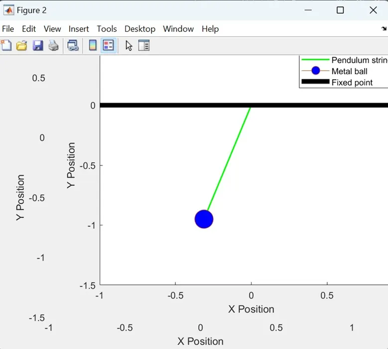
· plot([x0 x1], [y0 y1],'g', 'LineWidth',1.5); This line creates a plot that represents the trajectory of the pendulum string. It plots a green line segment from the point (x0, y0) to (x1, y1) with a linewidth 1.5.
· hold on This command tells MATLAB to keep the current plotin the figure and allow additional plots to be added to it.
· plot(x1,y1,'Marker','o','MarkerSize',20,'MarkerFaceColor','b') This line creates a plot that represents the position of the metal ball at its current coordinates (x1, y1).
o Marker: Specifies the type of marker used to represent data points.
o MarkerSize: Sets the size of the marker. In this case, sets to 20, making the circular marker relatively large.
o MarkerFaceColor: Determines the color of the marker’s face. It’s the set to ‘b’ indicating that the marker’s face is filled with the blue color.
· xlabel('X Position') and ylabel('Y Position') This lines set the labels for the x-axis and y-axis, respectively.
· title ('Pendulum Trajectory') This line sets the title of the plot to “Pendulum Trajectory”.
· plot([-1 1 ],[0,0],'color','black','LineWidth',5) This line creates a horizontal black line segment at y = 0, which represents the equilibrium position of the pendulum. The line width has 5.
· axis([-1 1 -1.5 0.5 ]) This line sets the axis limits for the x and y axis, controlling the viewable portion of the plot.
· legend('Pendulum string', 'Metal ball','Fixed point'); This line adds a legend to the plot, labelling the green lines as “Pendulum strings”, the blue marker as “Metal ball”, and the black horizontal line as “Fixed Point”.
· pause(0.01) This line introduces a b rief pause of 0.01 seconds. It can be useful when you want to animate the pendulum’s motion, allowing you to see the motion over time.
· hold off This command turns off the “hold off” mode, so any subsequent plots will not be added to the current figure. It resets the figure for the next frame in an animation or additional plots.
M(i) = getframe(gcf);
· The code M(i) = getframe(gcf); is used in MATLAB to capture and store frames from a figure for the purpose of creating animations or recording the sequence of frames.
movie(M)
videofile = VideoWriter('Sec_Order_ODE', 'Uncompressed AVI');
open(videofile)
writeVideo(videofile,M)
close(videofile)
· movie(M) This function used to play back the sequence of frames stored in the ‘M’ array. It displays the frames as animation on the screen. The frames in ‘M’ are shown one after the other in quick succession to create the animation.
· videofile = VideoWriter('Sec_Order_ODE', 'Uncompressed AVI'); This line sets up a VideoWriter object named videofile. This object will be used to write and save the animation as video file. The first argument Sec_order_ODE specifies the name of the video file you want to create and the second argument Uncompressed AVI indicates type of video file format to be used.
· open(videofile) This function opens the video file specified by the VideoWriter object for writing. It prepares the video file for receiving the frames of the animation.
· writeVideo(videofile,M) This function write the frame stored in the M array too the video file specified by the VideoWriter object videofile.
· close(videofile) This function closes the video file, finalizing the video writing process and making the video file complete and ready for use.
function dtheta_dt = ode_func(t ,theta,b,g,l,m)
theta1 = theta(1); % Extract the first angle from the input
theta2 = theta(2); % Extract the second angle from the input
dtheta1_dt = theta2; % First derivative of theta1
dtheta2_dt = -(b/m)*theta2 - (g/l)*sin(theta1); % Second derivative of theta
dtheta_dt = [dtheta1_dt; dtheta2_dt]; % Combine the derivative into a column ve
· function dtheta_dt = ode_func(t ,theta,b,g,l,m) This line declares a function named ode_func that takes six input arguments (‘t’, theta, b, g, l, and m). It is meant to be used as the right-hand side of an ODE solver.
· theta1 = theta(1); and theta2 = theta(2); These lines extract the components of the state vector theta into separate variables. theta1 corresponds to the angle of the pendulum, theta2 corresponds to the angular velocity of the pendulum.
· dtheta1_dt = theta2; This line calculates the derivative of the angles (theta1) with respect to time, which is simply the angular velocity (theta2). It is the first component of the derivative vector.
· dtheta2_dt = -(b/m)*theta2 - (g/l)*sin(theta1); This line calculates the derivative of the angular velocity (theta2) with respect to time.
o Damping term -b/m*theta2 where b is a damping coefficient and m is the mass of the pendulum.
o Gravitational term –(g/l)*sin(theta1) where g is the acceleration due to gravity and l is the length of the pendulum. The negative sign indicates that it’s acting in the opposite direction to the angle of the pendulum.
· dtheta_dt = [dtheta1_dt; dtheta2_dt]; This line assembles the derivaties of the angle and angular velocity into a column vector dtheta_dt. The ODE solver will use this vector to update the state of the pendulum overtime.
Output:
Results:
https://drive.google.com/file/d/1MuxRwYIdENrqIC0zGE9IddZmHajFu4qb/view?usp=sharing
Conclusion:
This process provides valuable insights into the behavior of a simple pendulum, the impact of its parameters, and the principles of numerical simulation and animation.
In the simulation, we consider a pendulum with the length of 1meter, a mass of 1kg, damping coefficient of 0.05, and gravitational acceleration of 9.81m/s^2. We simulate its motion over a time span of 0 to 20 seconds, with initial conditions of an angular displacement of 0 radians and an angular velocity of 3rad/s at time t = 0.
The simulation allows us to understand how the penduluum’s angle changes over time, visulaizing its oscillatory motion. By animating the pendulum, we can further enchance our understanding and create a visual representation of the physical phenomenon.
In conclusion, simulating pendulum motion in MATLAB by the provided challenge, is a practical excersice that offers hands-on experience in solving differential equations, exploring dynamic systems and creating visulizations. This kind of excersice is invaluable for learning and teaching the principles of physics, numerical methods and dynamic modelling.