Week 4.1: Project - Steady state simulation of flow over a throttle body

Aim:

Set up and run the steady-state simulation for flow over the throttle body.

Objectives

• Post-process the results and show pressure and velocity contours.
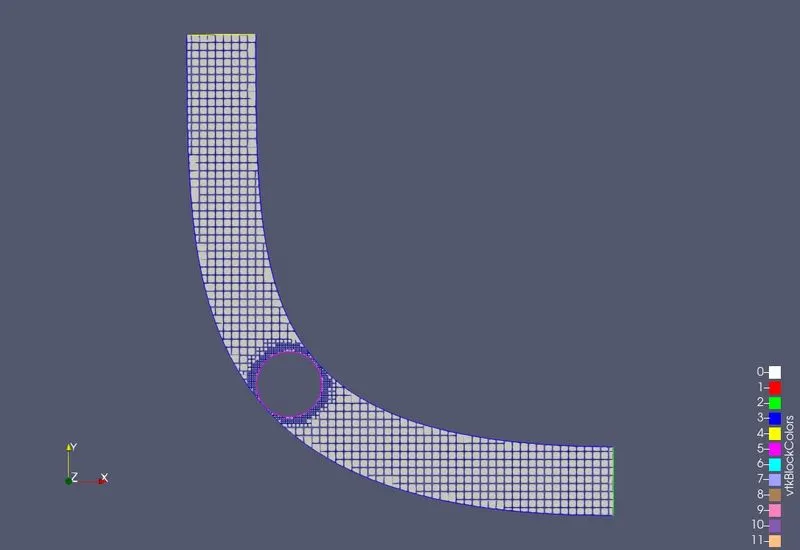
• Show the mesh (i.e surface with edges)
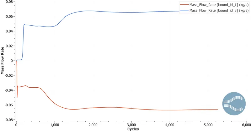
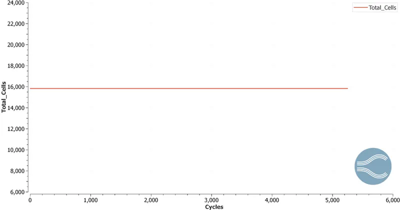
• Show the plots for pressure, velocity, mass flow rate and total cell count.

Methodology

Here flow properties when air flows through a throttle body are studied using CONVERGE CFD with the help of CYGWIN and ParaView. The geometry is imported from a 3d file. The dimensions are in meters.

To create the geometry and to set up the problem, Converge studio is used.

To simulate the problem, CYGWIN is used.

To post-process the results ParaView and converge are used.

Throughout the simulation, the flow is considered to be steady and turbulent.

• Pre-processing

Model Creation

After opening converge studio import the 3D part file.

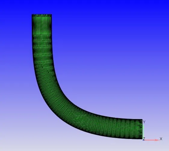
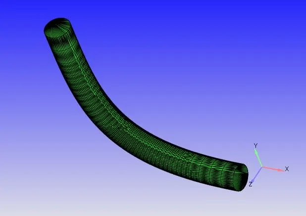
Remove all the unwanted surfaces in the geometry and close all the open edges.

The next step is to create boundaries by grouping the triangles. Go to boundaries, click on the flag and make the boundaries as required.

Here 4 boundaries are created, inlet, outlet, wall, and throttle. The throttle is inside the wall which is not visible in the following image.

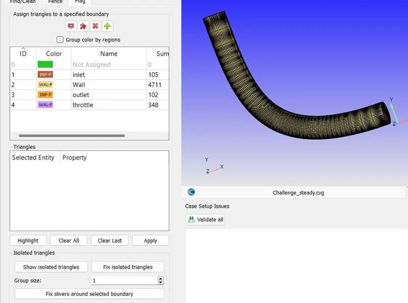
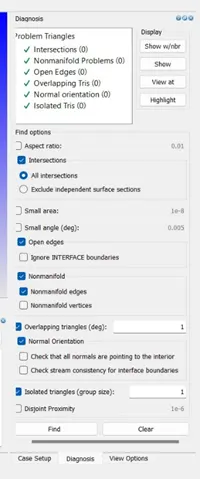
Enable the normal vectors to see whether the normals are pointing towards the fluid region. To run the simulation, the normals should point towards the fluid region. If it is not, click on transform, go to normal, select the triangle, and click on apply. Now the normals are pointed towards the fluid region. To check for any errors in the geometry, go to diagnosis and click on find. If all the items are green then the geometry is clean and we are ready to proceed with case setup.

Case setup

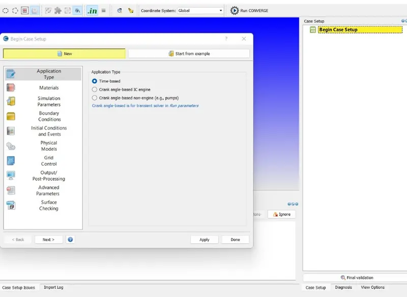
Click on begin case setup under case setup. Since we are not dealing with the IC engine problems, select Time based and click Apply.

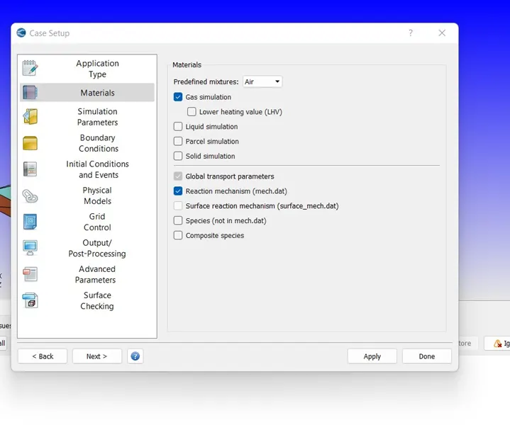
Now converge will give access to edit all the simulation setups. Now click on materials to assign material. Select Air as material. Since we are not interested in species uncheck species and click on apply.

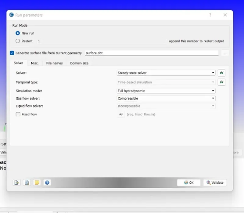
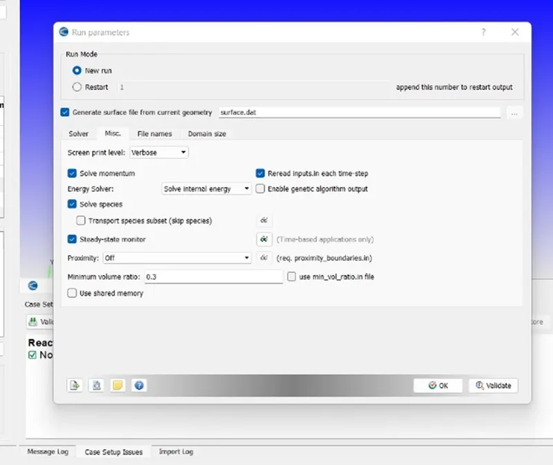
Validate gas simulation and global transport parameters and move on to run parameters. Change the solver to a steady-state solver. Under the misc tab, check the steady-state monitor and uncheck use shared memory. Click on ok and for load recommended defaults click cancel.

Next, we will define the fluid region and initialization parameters by clicking on regions and initialization. Click on add and create a region. Select air as species in that region and click on ok.

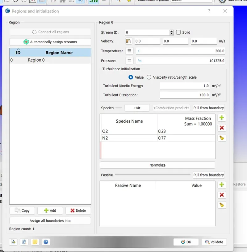
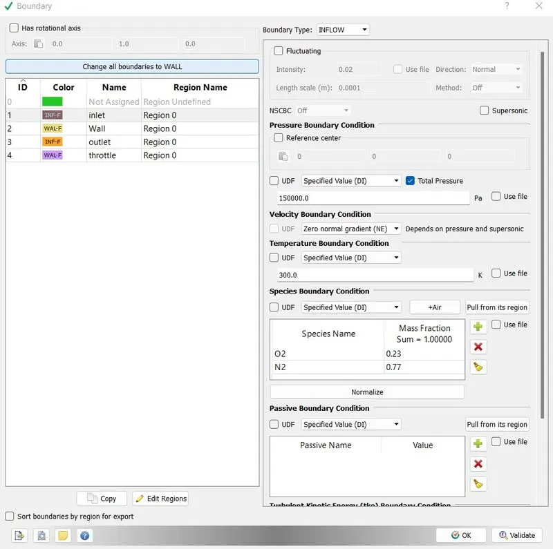
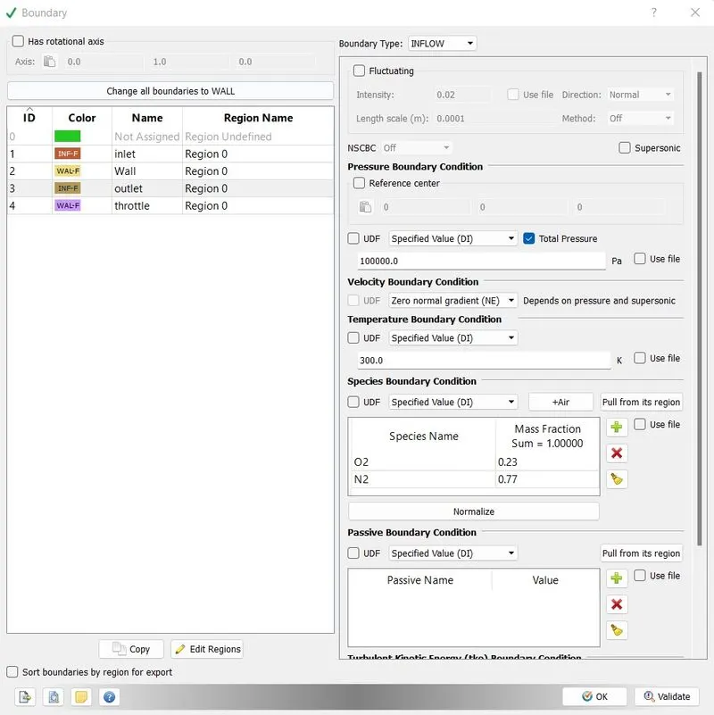
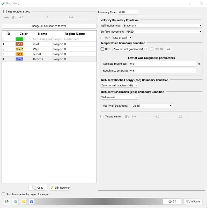
After defining the regions go to boundary to define the boundary conditions. The following boundary conditions are used, and select the above defined region as region for all BC.

Inlet – INFLOW

Specified value = 150000 Pa

Temperature = 300 k

Species = Air

Outlet – OUTFLOW

Specified value = 100000 Pa

Temperature = 300 K

Backflow species = Air

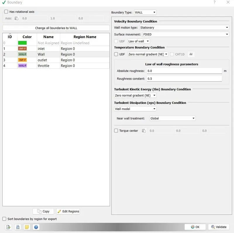
Wall – WALL

Law of wall

Temperature = 300 K

Zero normal gradients (NE)

Throttle - Wall

Law of wall

Temperature = 300 K

Zero normal gradient (NE)

Since we are dealing with turbulent flow, select RNG k-epsilon from turbulence.

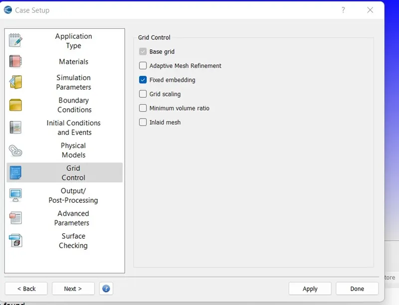
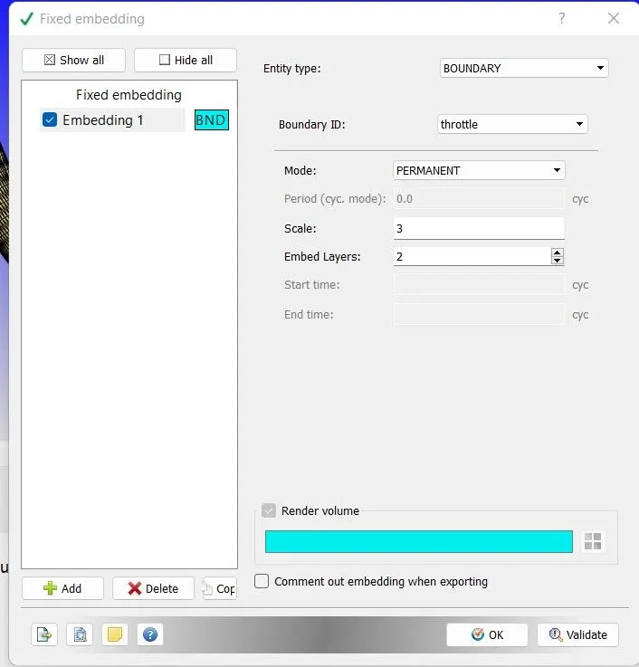
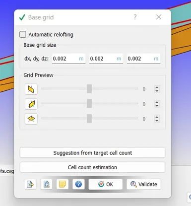
Grid sizes are changed as per the case setup defined in the methodology. We go for fixed embedding in grid size options. Click on add, select BOUNDARY as entity type, select wall and select permanent as mode.

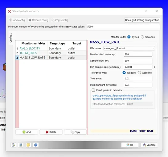
The following changes were made in steady state monitor. The solver will run at least for 5000 cycles even if the solution gets converged before.

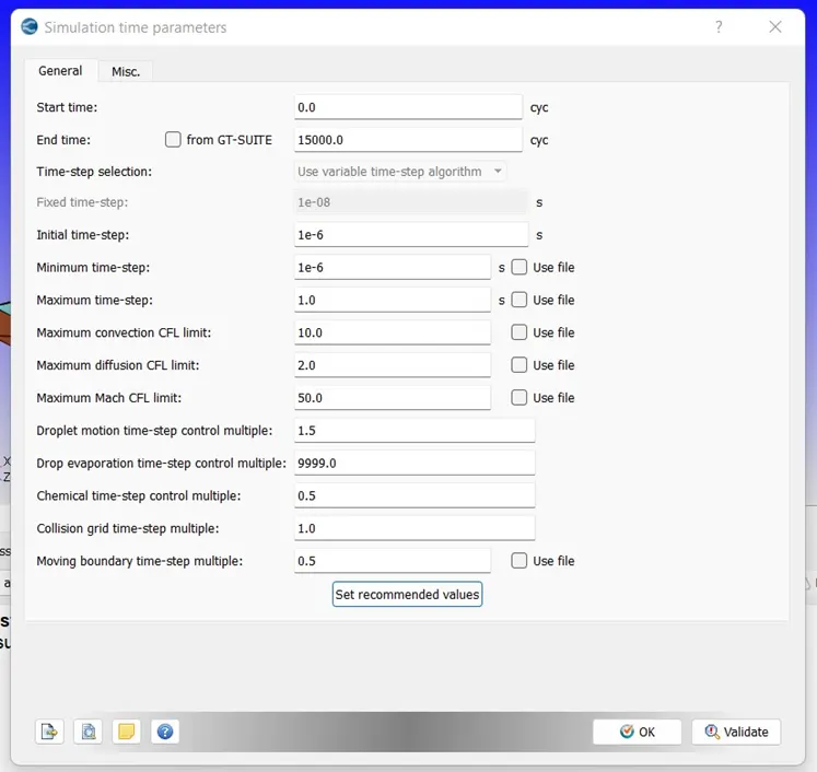
The simulation is set to run for 15000 cycles with the following time parameters.

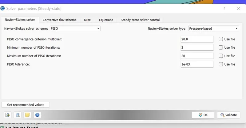
Under solver parameters, change solver type to pressure-based solver

Select all the required variables required from the Post variable selection and click on ok.

Another important thing to note is the time interval for writing the 3D output data files. There should be at least 100 output files available by the end of the simulation. So the number of intervals should carefully be given. We will be keeping 100 as an interval. So for 15000 cycles, there will be 150 output files. For this, click on output files and navigate to writing time intervals. Give 100 cycles at a time interval for writing 3D output data files.

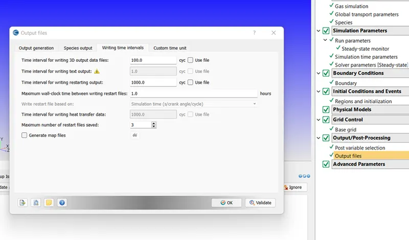
Click on final validate to validate all the setup. If all are fine, converge will say that no issues were found.

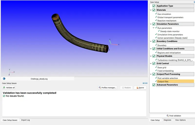
Now go to file then click on export and click on export input files to export the setup files. Save these files to Cygwin run folder to make the simulation to run through CYGWIN.

The simulation is run using CYGWIN interface and the results were then converted to binary form using CONVERGE so that ParaView can understand the result data and post-process it.

Results and Discussion

1. Mesh
   
   
   
2. Velocity contour-vector plot
   
   
   
   
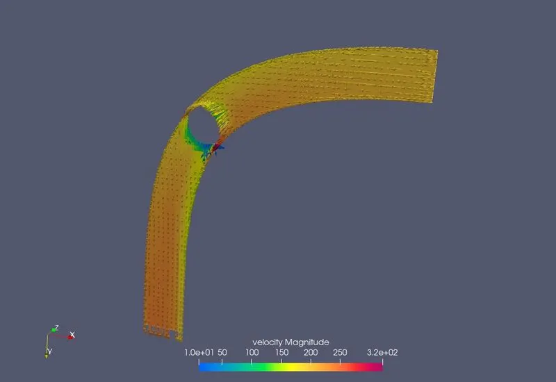
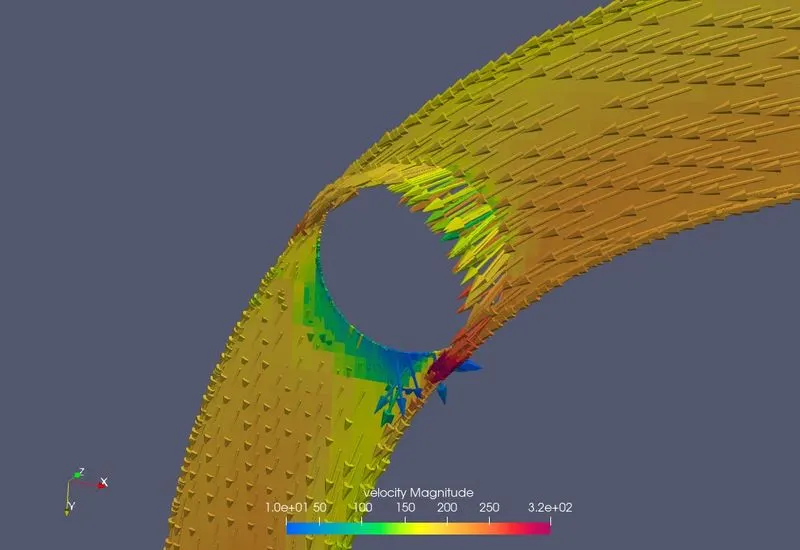
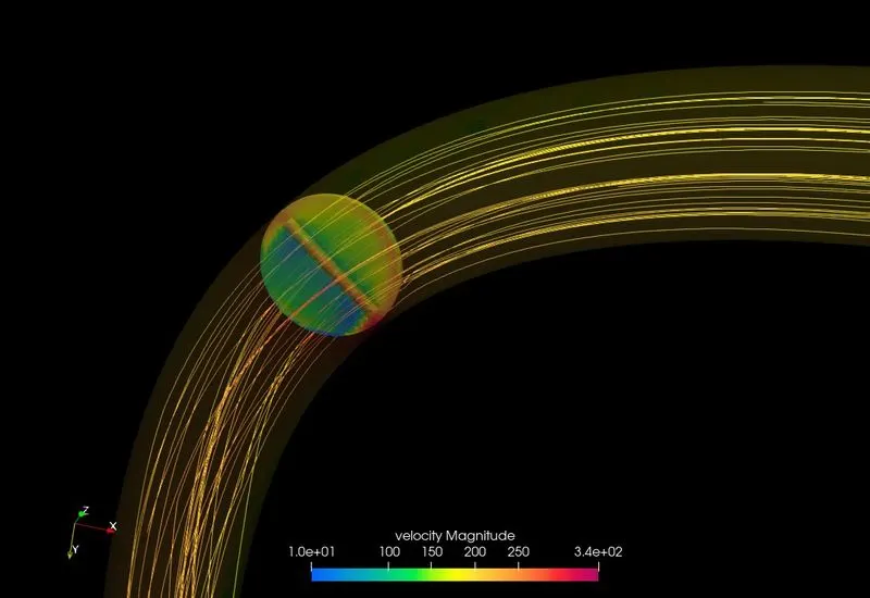
3. Velocity contour-streamline plot
   
   
   
   
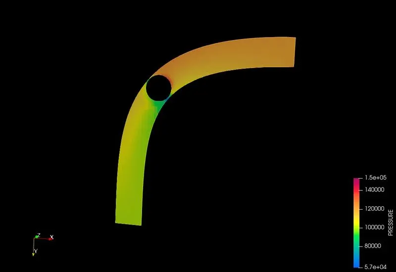
4. Pressure contour
   
   
   
   
5. Velocity contour – Animation
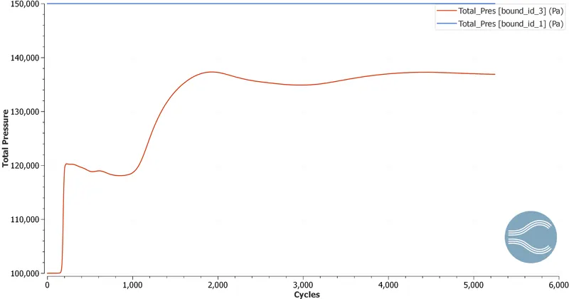
   https://drive.google.com/file/d/1LyueLK1SF8SD76jeLTRVbC24tj0JaF2J/view?usp=sharing
   
   
6. Total Pressure
   
   
   
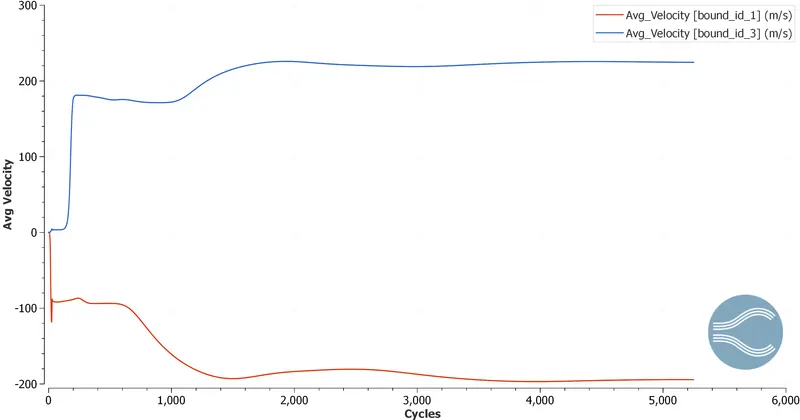
7. Average velocity
   
   
   
8. Massflow rate
   
   
   
   
9. Cell count
   
   
   
   
   
   

   Conclusion

   • The velocity contour shows the velocity distribution throughout the flow region. Just after the throttle, we can observe the formation of wake regions.
   • Since the throttle is at a maximum open position, the maximum amount of fluid passes through the throttle.
   • We can observe a pressure build-up on the fluid strike face of the throttle in the pressure contour. As it passes over the throttle, the pressure decreases and the velocity increases and the fluid passes over the throttle region by creating a wake region just behind the throttle body.
   • It is clear from the mass flow rate plot that the mass flow rate at the inlet is the same as at the outlet.
   • The total pressure plot indicates that the outlet pressure is increasing to reach up to the inlet pressure.
   • The attached animations give a clear visualization of the flow field throughout the simulation. It clearly shows Separation also.