Steady state simulation of flow over a throttle body

I. Aim: 3D CFD analysis of flow over a throttle body in a pipe elbow using Converge CFD.

II. Problem Statement: Perform 3D steady-state flow over a throttle body in a pipe elbow geometry using a suitable solver available in Converge CFD. The case setup is done using ConvergeCFD and simulation is run in the CYGWIN terminal. Further, post-processing is done using Converge CFD and ParaView. The main objective of this project is to simulate a simple case of obstruction to flow caused due to throttling and its effect on mass flow rate in the domain using ConvergeCFD.

III Objectives:

1. Simulate 3D steady-state flow over a throttle body in a pipe elbow using ConvergeCFD and CYGWIN terminal.

2. Postprocess results in ParaView and ConvergeCFD and report the following:

- Velocity and pressure contours

- Show mesh (i.e surface with edges)

- Plots for velocity, pressure, mass flow rate, and total cell count.

IV: Solving & Modelling approach:

3D steady-state CFD analysis of flow over a throttle body in a pipe elbow case is set up in ConvergeCFD and then running the solution in CYGWIN terminal. Air is used as the fluid flowing through the channel (77% N2 and 23%O2). Postprocessing is done using ConvergeCFD and ParaView. Three meshes are used to check the effect of cell size on the results.

1. Geometry/Domain:

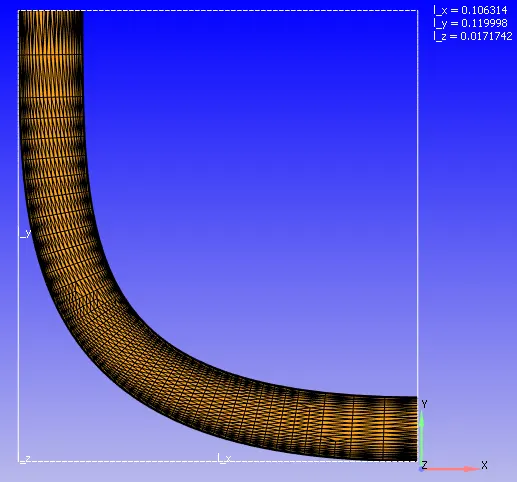
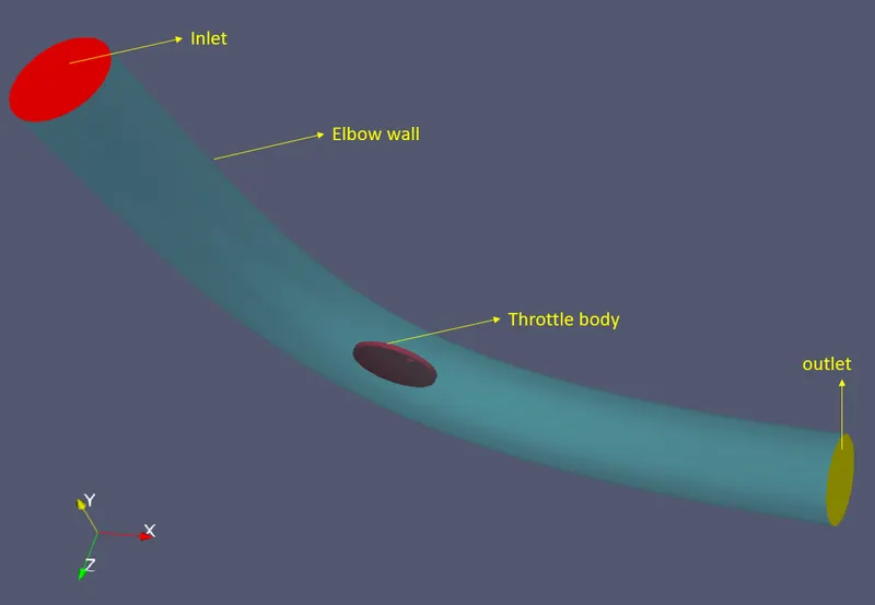
A 3D solid geometry (.stl file) of the typical pipe elbow with a throttle body (valve) is imported into ConvergeCFD. The following figure shows the imported geometry scaled by 0.001 value. In ConvergeCFD triangles are the basic building blocks. Hence the surfaces of the geometry are a combination of triangles. The geometry is then simplified by removing the outer walls. The bounding box dimensions of the scaled-down geometry are also shown in the following figure:

2. Boundary Flagging:

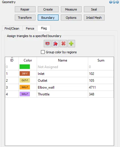
The boundary zones in ConvergeCFD are created by flagging boundaries. This can be done by creating boundary flags in the boundary tab as shown below:

3. Case setup:

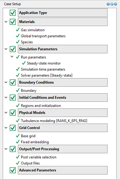
After assigning boundary zones as mentioned above, the solution case setup is to be done. ConvergeCFD has a dedicated menu to completely set up the solution. Details are as follows:

-In the application type option, Time-based is selected.

- The materials option are selected as shown in below images:

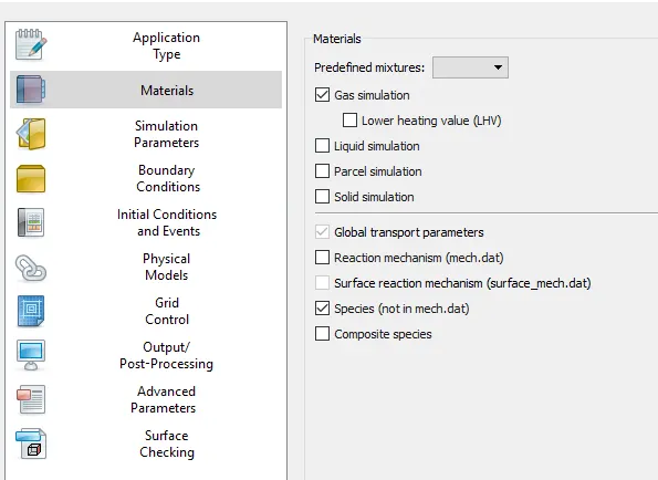
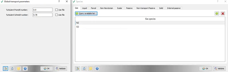
Air is chosen as the working fluid with 77% N2 and 23% O2.

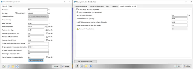
- Simulation Parameters:

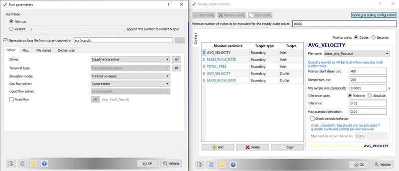
The steady-state solver option is selected and respective monitors for various flow variables are selected to monitor during the solution process.

- Boundary Conditions:

The boundary conditions are assigned to the respective boundary zones in this menu. The applied boundary conditions are as follows:

Boundary Zone	Boundary condition
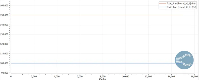
Inlet	Inflow -Total Pressure = 1.5E5 Pa, -Velocity = Zero normal gradient -Temperature = 300 K - Species - O2 = 0.23, N2 - 0.77
Outlet	Outflow - Pressure = 1E5 Pa -Velocity = Zero normal gradient - Temperature backflow = 300 K - Species - O2 = 0.23, N2 - 0.77
Elbow_wall	Wall - Stationary, Law of wall, zero normal gradient temperature. - Turbulence K.Energy = Zero normal gradient - Turbulence K.Dissipation = Wall model, Standard wall function
Throttle	Wall - Stationary, Law of wall, zero normal gradient temperature. - Turbulence K.Energy = Zero normal gradient - Turbulence K.Dissipation = Wall model, Standard wall function

The above boundary conditions can be defined only after defining a region in the Initial conditions and Events section of the case setup as shown below:

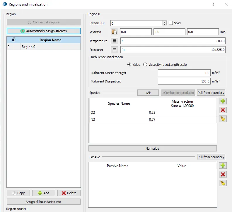
The turbulence in the flow is modeled using the RNG-K-ε RANS model with standard wall function as shown below:

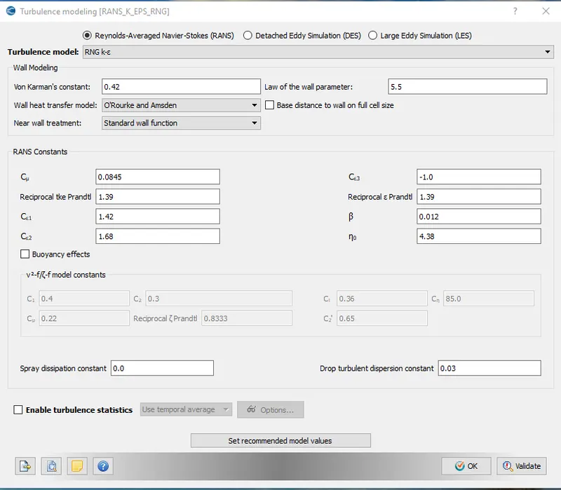
- Grid control:

The mesh size for the domain is defined in this tab as shown below:

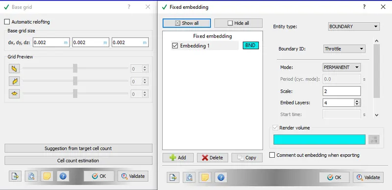
The fixed embedding option is turned on to increase the cell count around the throttle body outer walls to accurately capture the boundary layer near the throttle body.

The mesh sizing considered in this analysis are as below:

• default mesh dx = dy = dz =2e-3 m
• Embedding on throttle body walls: Entity type = Boundary, Mode = Permanent , Scale = 2, Embed layers = 4

- Output and post-processing:

The flow variables of interest, which are to be post-processed after the solution are selected in this option, and also at how many intervals these are written to the output file.

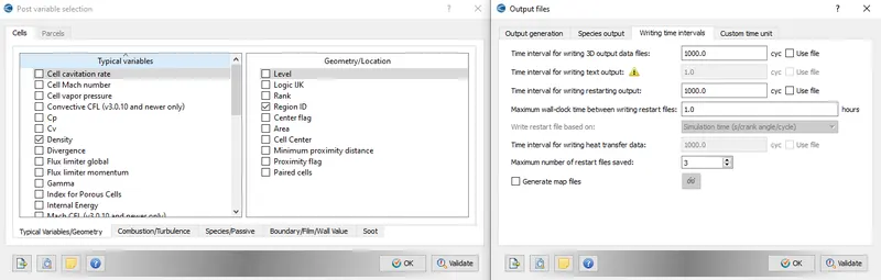
After all the above setup is completed final validation option is selected to check for the case setup is free of setup errors. After validation, the case setup files are exported using the export option in the File menu to the working folder. These files will be used by the CGYWIN terminal to run the solution. The above process is repeated for all the mesh sizes and the respective setup files are exported.

Solution in CYGWIN :

The solution is run in the CYGWIN terminal. First, we have to navigate to the respective working folder in the CYGWIN terminal, where case setup files are present. Then by executing the following command, the solution can be run:

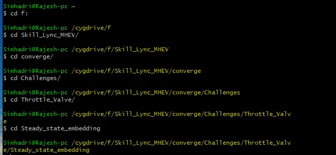
Executing the converge.exe using 4 parallel processors to run the solution:

The solution will run-up to the number of cycles set in the run setup and the output files are saved to the respective folders.

V Post-Processing Results:

After the solution is complete, post-processing of the results is done using CONVERGE CFD and ParaView.

The plots are plotted in CONVERGE CFD, whereas to visualize the flow variables using contour plots the output files need to be converted to ParaView compatible files. This can be done in the CONVERGE CFD Post-Processing 3D tab as shown below:

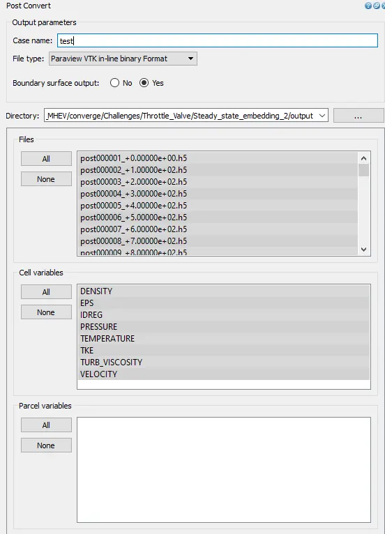
Visualization in ParaView:

The converted ParaView compatible output files are opened in ParaView and the grid, contour plots for Pressure, Velocity, and velocity streamlines are visualized:

Grid:

Whole geometry (3D)	Central cut plane (2D)

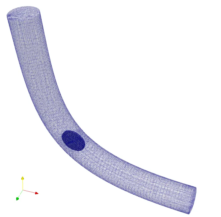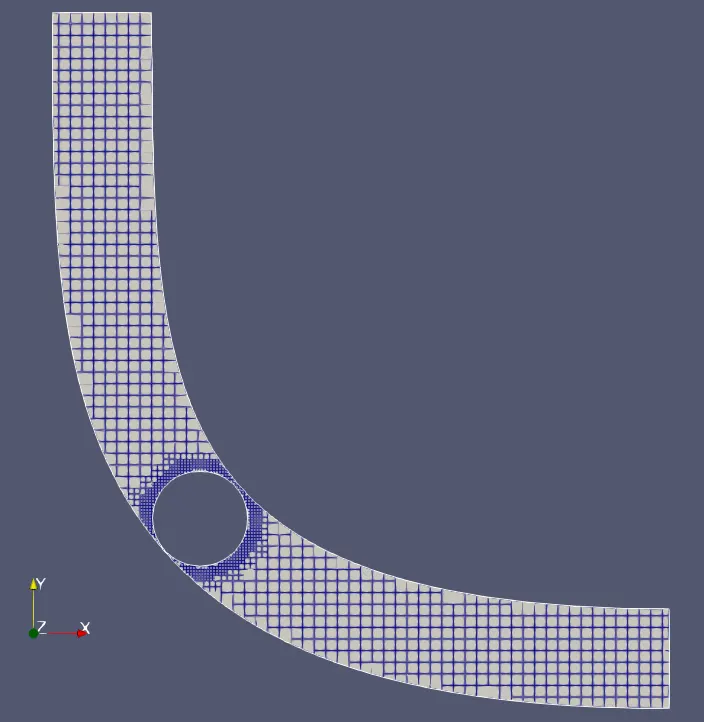The above figures show the mesh generated with fixed embedding around the Throttle body. The mesh refinement around the Throttle body is required to capture the turbulence effects.

Contour plots in 3D:

Velocity:

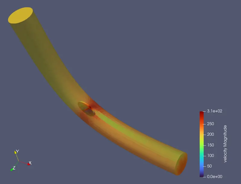
The above contour plot shows the velocity variation in the elbow, with maximum velocity observed around the throttle body because flow area is reduced due to the presence of the throttle body.

Pressure:

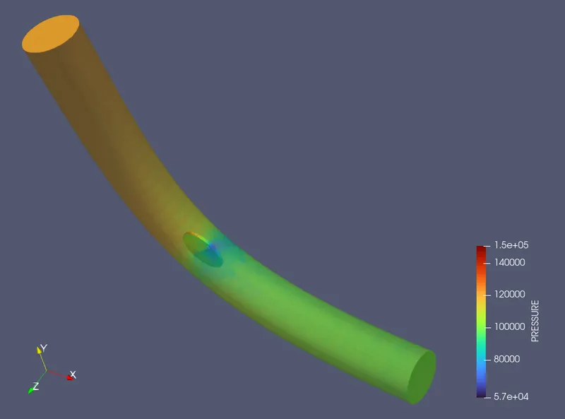
Velocity Streamlines in the domain along with pressure contours on the Throttle body:

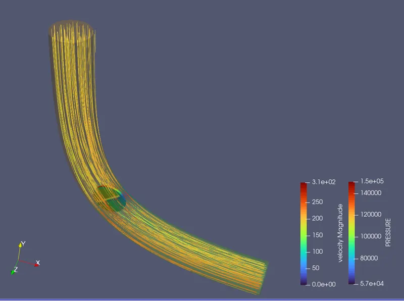
The above contour plot shows the velocity streamlines in the elbow along with the pressure contour on the throttle body.

Velocity contour at a central cut plane (2D):

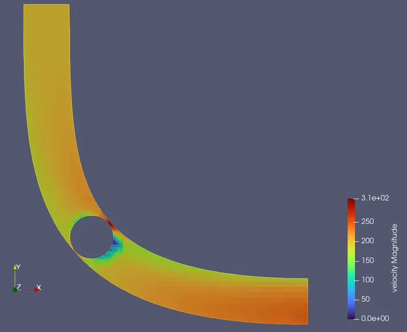
The above contour plot represents the velocity distribution at the central cut plane of the domain in 2D. It can be clearly seen that a zero velocity region (wake/void) formed behind the throttle body due to flow separation.

Pressure contour at a central cut plane (2D):

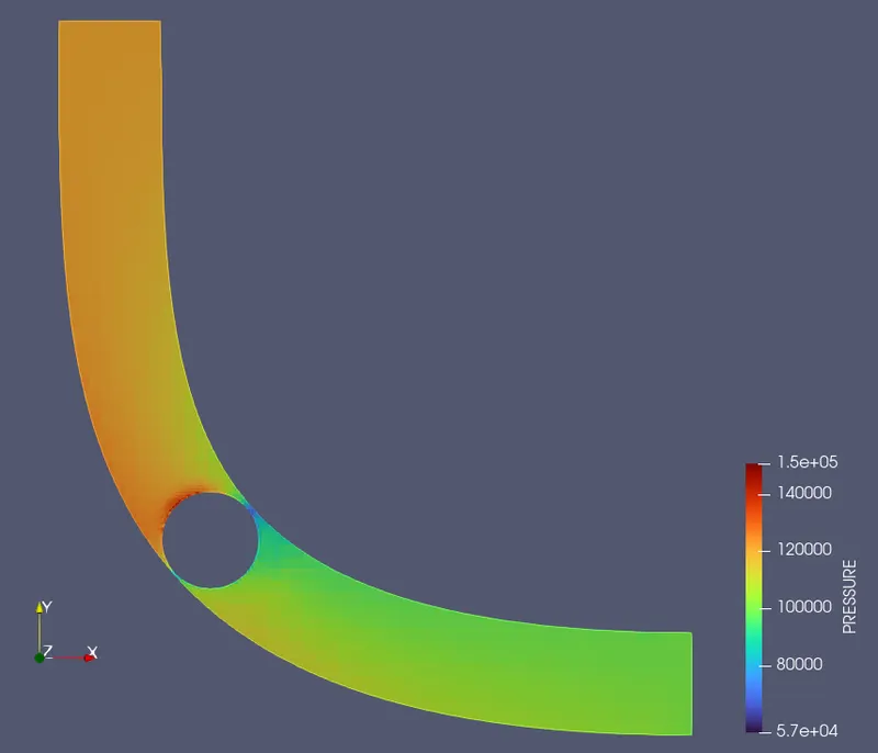
The above contour plot represents the pressure distribution at the central cut plane of the domain in 2D. It can be clearly seen that a high-pressure region formed in front of the throttle body due to flow stagnation and kinetic energy converted to pressure energy.

Graph plots in Converge CFD:

The graphs are plotted for various flow variables using the line plotting tab in Converge CFD:

Cell count:

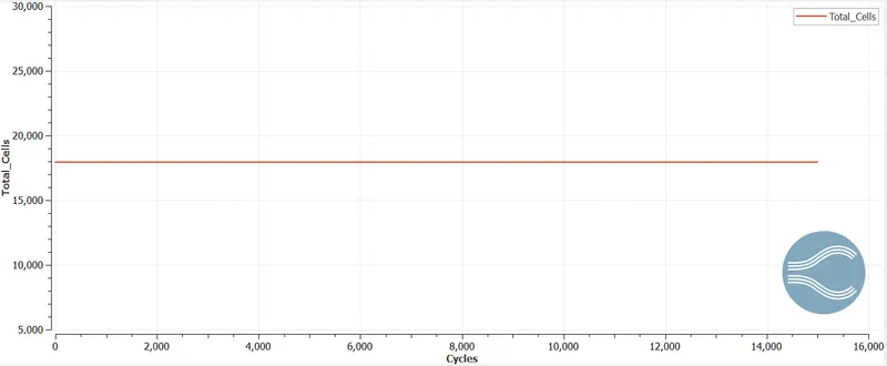
Pressure at inlet(bound_id_1) and outlet (bound_id_2) :

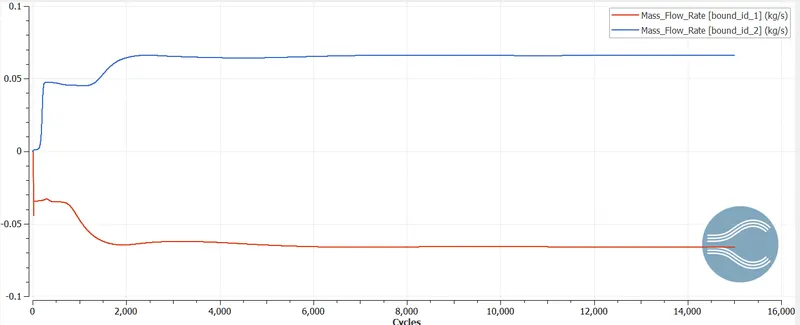
Mass flow rate at inlet(bound_id_1) and outlet (bound_id_2) :

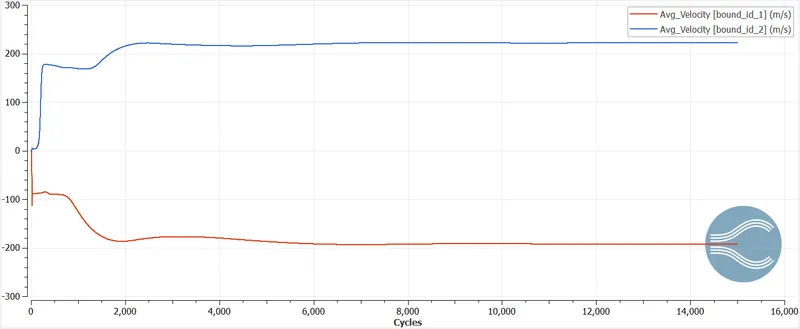
Average Velocity at inlet(bound_id_1) and outlet (bound_id_2) :

Conclusion:

In this project, the basic Steady-state case setup in ConvergeCFD along with turbulence modeling, running the setup in CYGWIN terminal, and post-processing in ParaView, Converge CFD is carried out for flow over a throttle body in an elbow type flow geometry. The effect of the throttle body on the flow stagnation, wake created due to the flow separation is studied using the RANS RNG k-ε">ε turbulence model. Further study can be done with varying throttle body opening angle and analyzing its impact on the flow dynamics using transient analysis.