Solving second order ODE of Simple Pendulum motion using MATLAB

I: Aim & Introduction:

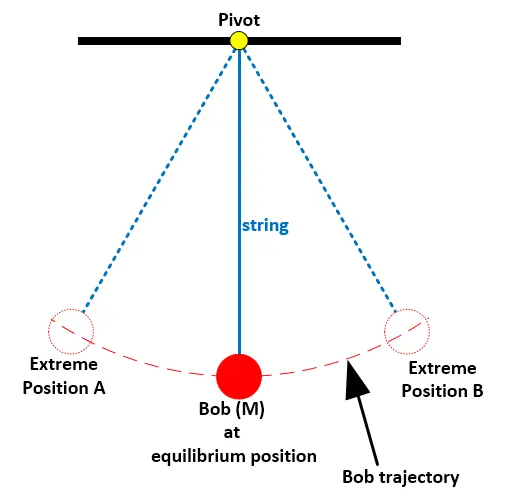
The aim of this project is to solve the second-order ODE of the simple pendulum motion. A simple pendulum is a system that comprises of a heavy mass(bob) attached to a massless string and pivoted at the top as shown in Figure1.

(a)	(b)

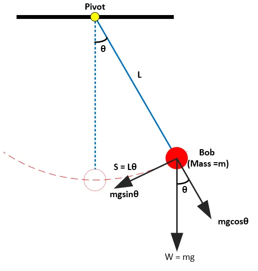
Figure1: Simple Pendulum

When the pendulum is given as initial angular displacement from its equilibrium position, it oscillates to and fro as shown in Figure1(a). The motion is in a single plane. Consider a simple pendulum system as shown in Figure1. It consists of a bob of mass ‘m’, attached to a string of length ‘L’, and pivoted at the top end. The pivot is a frictional pivot and hence provides damping to the motion of the pendulum. θ is the angular displacement. The forces acting on the pendulum are the weight of the bob, the inertia forces and the frictional damping force. Since the pendulum motion is along a circular path(trajectory), the acceleration and velocity can be considered in tangential directional only. In order for the pendulum to remain in its equilibrium, the forces acting on it should be conserved(F_total = 0).

The total force acting on the pendulum is:

F_total = F_inertia + F_damping +mgsinθ

Where,

F_{inertia =} is the force due to acceleration along the tangential direction

F_damping is the damping force due to friction at the pivot

mgsinθ is the weight component along the tangential direction

Since (S=Lθ) is the arc length traversed by the bob the angular velocity and acceleration in tangential direction are given by;

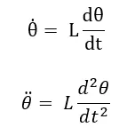
Therefore,

`mL (d^2 θ)/(dt^2 )+bL (dθ)/(dt)+mgsinθ=0`

Simplifying above equation leads to;

`(d^2 θ)/(dt^2 )+b/m (dθ)/(dt)+g/L sinθ=0` (1)

Equation (1) is the governing equation of motion of simple pendulum with damping.

The second-order differential equation of simple pendulum motion is solved using the ‘ode45’ solver in MATLAB to visualize the pendulum oscillatory motion.

II. Objectives:

1. Write a program to solve the second-order ode of a simple pendulum motion.
2. To animate the pendulum oscillatory motion and to create a movie.

III. Program:

The program is written in MATLAB. The code is as shown below:

%program to animate the motion of a simple pendulum
clear all
close all
clc


%pendulum properties
g = 9.81;           %acceleration due to gravity in m/s^2
L = 1;                %length of the massless string considered in m
m = 1;                  % mass of the bob attached to the string in kg

b = 0.05;               %damping(air resistance) considered in N/m


t_total = linspace(0,20,400); %total time period of the pendulum: 20 s.

%initial conditions
theta0_omega0 = [0;3];         %initial angular displacement is zero and angular velocity is 3 rad/sec


%computing angular displacemnts and velocities an array by calling the pendulum_ode function with appropriate input arguments
[t,results] = ode45(@(t,theta) pendulum_ode(g,b,L,m,t,theta),t_total,theta0_omega0);  %array containing the angualr displacements and velocities traversed by pendulum for the total time of 20 sec

disp_ang= results(:,1);   %vector containing the angualr displacement values traversed by pendulum for the total time of 20 sec
velocity_ang = results(:,2);     %vector containing the angualr velocity values traversed by pendulum for the total time of 20 sec

%plotting the dynamics of the pendulum
figure(1)         %Figure/graph storing the dynamics of pendulum 
plot (t,disp_ang)   %plotting the angular displacements with respect to time
hold on
plot(t,velocity_ang)     %plotting the angular velocities with respect to time
hold off
%giving labels to axes, title, and legend for the above plot
xlabel('Time (s)')  
ylabel('Amplitude')
title('Dynamics of Simple Pendulum')
legend('angular displacement (radians)','angular velocity (rad/s)')


%to visualize the motion of pendulum and to animate it a for loop is written as shown below
K=1
for j = 1:length(t_total)           %looping in terms of  t_total values 
 
  x1=0;                             %x-coordinate of the fixed pivot end of pendulum
  y1=0;                             %y-coordinate of the fixed pivot end of pendulum
  x2= -L*sin(disp_ang(1:j));         %x-coordinate of the mass end of pendulum which is a function of string length andthe angular displacement and varies over time
  y2= -L*cos(disp_ang(1:j));            %y-coordinate of the mass end of pendulum whichis a function of string length andthe angular displacement and varies over time

  %plotting the motion of the pendulum
  figure(2)          %motion is plotted in Figure2                   
  plot([x1 x2(j)],[y1 y2(j)], 'color','b' ,'LineWidth',3)           %plotting the string as a line   
  hold on 
  plot(x2(j),y2(j),'o','MarkerSize',25, 'MarkerFacecolor','r','MarkerEdgecolor','r')  %plotting the mass as a sphere   
  line([-1 1],[0 0], 'LineWidth', 10, 'color', 'k')                 %to plot the edge on which the pendulum is pivoted
  %giving labels to axes, title, and legend for the above plot
  xlim([-1.1,1.1])
  ylim([-1.1,0.5])
  xlabel('x-direction co-ordinates (m)')
  ylabel('y-direction co-ordinates (m)')
  title('Motion of the pendulum')

  pause(0.05)   
  
  hold off

  V(K) = getframe(gcf);
  K=K+1;
     
end

movie(V)
animation = VideoWriter('Simple_Pendulum_Oscillation.avi','uncompressed avi')
open(animation)
writeVideo(animation, V)
close(animation)

Code Explanation:

Step1: clear all – command to clear the workspace.

Step 2: close all – command to close all opened previous plots.

Step 3: clc – command to clear the command window.

Step 4: pendulum properties and damping coefficient are defined in this step.

Step 5: the total time period of motion of the pendulum is defined for 20 sec using linspace command in this step.

Step 6: Since, the pendulum governing equation is a second-order ODE, solving it MATLAB requires it to be converted into a first-order ODE and solving it by using the inbuilt solver ‘ode45’. ‘ode45’ solves the first order ODE numerically by Runge-Kutta method and gives an approximate solution. The syntax for the ‘ode45’ is given below:

[t,y] = ode45(odefun,tspan,y0),

where tspan = [t0 tf], integrates the system of differential equations y′=f(t,y) from t0 to tf with initial conditions y0. Each row in the solution array y corresponds to a value returned in column vector t.

To solve the second order ODE of simple pendulum a function pendulum_ode is defined to convert it to first order ode and then it is called in the ode45 with appropriate initial conditions and time span to get the angular displacement and velocities of the pendulum. The function is as follows:

function [dtheta_dt] = pendulum_ode(g,b,L,m,t,theta)
    theta1= theta(1);           
    theta2=theta(2);
    
    dtheta1_dt = theta2;
    dtheta2_dt = -b/m*(theta2)-g/L*sin(theta1)
    
    [dtheta_dt] = [dtheta1_dt;dtheta2_dt];
    

end

The above function is called in the main program using the ode45 solver command to get the angular displacement and velocities of the pendulum over the total time period. The syntax for the same is as below:

[t,results] = ode45(@(t,theta) pendulum_ode(g,b,L,m,t,theta),t_total,theta0_omega0)

Where, [t,results] is an array storing the angular displacement and velocities. (t,theta) represents the properties on which the solver result mainly depend on. pendulum_odeis the function with appropriate input arguments. t_total is the total time of integration of the ODE with the initial conditions theta0_omega0.

Step 7: The next step is to plot the dynamics of the pendulum using the plot command. The plot is made in figure(1).

Step 8: Animate the plot:

To visualize the pendulum motion over its time period of 20 sec a for loop is created to get the coordinates of the pendulum mass for each time increment. Then a plot of the pendulum is plotted in figure(2). The string is plotted as a line with appropriate color and line width.

The mass is plotted as a sphere with an appropriate color and marker size. The edge on which the pendulum is pivoted is plotted as a line. The plot at each time increment are stored in variable V(K) using the getframe command to create the animation. The extracted plot frames stored in variable V(K), are sorted into a single animation using the command movie(V).

Step 9:

The next step is to create an animation by using the VideoWriter command.

animation = VideoWriter('Simple_Pendulum_Oscillation.avi','uncompressed avi')

where, 'Simple_Pendulum_Oscillation.avi' is the filename and 'uncompressed avi' is the profile format.

Step10:

open(animation) - command used to open the animation file.

writeVideo(animation, M) - This command is used to write the frames in V(K) into the animation.

close(animation) - command used to close the animation.

IV. Errors during coding:

1. While calling the pendulum_ode function in the main program an error was observed and is as follows:

The error was the input argument L is not included while calling the function, whereas it was defined in the function program. The error is rectified by inserting the input argument ‘L’ in the main program while calling the function.

[t,results] = ode45(@(t,theta) pendulum_ode(g,b,L,m,t,theta),t_total,theta0_omega0);

2. While computing the co-coordinates of the mass an error was thrown in the command window as follows:

While computing the co-ordinates, a typo error was made by not inserting the ‘*’ operator. This was rectified by inserting the ‘*’ in the syntax as follows:

x2= -L*sin(disp_ang(1:j));

3. Error while plotting the string as a line.

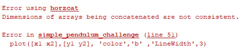
This error is due to defining x2 and y2 as single values, whereas they are actually dependent on time. The error is rectified by indexing the x2 and y2 in terms of time increment and the syntax for the same is given below:

plot([x1 x2(j)],[y1 y2(j)], 'color','b' ,'LineWidth',3)

4. Unrecognized function or variable ‘writevideo’.

The error is due to a syntax error for writing the video command. The error is rectified as below:

writeVideo(animation, V)

V. Output:

The output of the above program are the dynamics of the pendulum and the pendulum oscillatory motion.

1. Dynamics of the Pendulum:

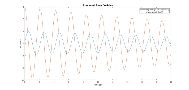
The above represents the dynamics of the pendulum in terms of angular displacement and velocities over time. The plot represents the dynamics for a time period of 20 sec. It can be observed that the displacement and velocities amplitudes are in the form of sine-waves. Hence the motion of the pendulum is a simple harmonic motion. The angular displacement and velocities start at 0 radians and 3 rad/s respectively, which are the initial conditions given for solving the ODE. Also, it can be inferred from the plot that the amplitude reduces for successive time increments. This is due to the frictional damping effect included in the governing equation of the motion.

2. Simple Pendulum Oscillation Animation:

The oscillatory motion of the simple pendulum is shown in the animation. It can be seen that the pendulum is pivoted at the top and oscillates to and fro along the tangential direction in a single plane. The blue line represents the string and the red sphere represents the bob. Also,the oscillation reduces over time due to the damping effect.