Deriving 4th order approximation of a 2nd order derivative using Taylor Table method
I. Aim:
To Derive the 4th order approximations of the second-order derivative of a function for the following numerical schemes.
1. Central difference
2. Skewed right-sided difference
3. Skewed left-sided difference
Numerical schemes:
1. Fourth order Central difference approximation of the second-order derivative of a function:
Consider a function f(x) whose numerical approximated second-order derivative is given by :
`f’’(x) =(δ^2 f)/(δ^2 x)`
The order of accuracy for the central difference method is found as:
P = N - Q + 1
Where,
P is The order of accuracy
N is the number of nodes in the stencil
Q is the order of derivative
Therefore the number of nodes to be considered for a fourth-order accurate approximation of a second-order derivative by central difference method is given by:
4 = N -2+1
N = 5.
For a central difference method, a function at a node can be evaluated by considering the information on both sides in the numerical stencil. Hence the numerical stencil of a function f(x) with fourth-order approximation with 5 nodes at appointing ‘i’ can be represented as:

Let the hypothetical second order derivative of function f(x) at ‘i’ considering the fourth order central difference approximation in terms of information from surrounding nodes be written as:
`(δ^2 f)/(δx^2 ) ≅ a* f(i-2) +b*f(i-1) + c*f(i)+d*f(i+1) +e*f(i+2)` .......(1)
Where a, b, c, d, e are coefficients of approximations.
Let ‘dx’ be the discretization size , then from Taylor series expansion of the first term a* f(i-2) gives,
`a×f(i-2)=a [f(i)-(f’(i)(2dx))/1!+(f’’(i) (2dx)^2)/2!-(f’’’(i) (2dx)^3)/3!+(f^(IV )(i) (2dx)^4)/4!-(f^V (i) (2dx)^5)/5!+(f^(VI)(i) (2dx)^6)/6!+⋯]`
Simplifying the above equation,
`a×f(i-2)=a f(i)-2af’(i)dx+4a/2 f’’(i) (dx)^2-8a/6 f’’’(i) (dx)^3+2a/3 f^(IV) (i) (dx)^4-4a/15 f^V (i) (dx)^5+4a/45 f^(VI) (i) (dx)^6+…`
Similarly taylor series expansion of the second term b* f(i-1) gives,
`b×f(i-1)=b f(i)-bf’(i)dx+b/2 f’’(i) (dx)^2-b/6 f’’’(i) (dx)^3+b/24 f^(IV) (i) (dx)^4-b/120 f^V (i) (dx)^5+b/720 f^(VI )(i) (dx)^6+...`
Similarly taylor series expansion of the fourth term d* f(i+1) gives,
`d×f(i+1)=d f(i)+df’(i)dx+d/2 f’’(i) (dx)^2+d/6 f’’’(i) (dx)^3+d/24 f^(IV) (i) (dx)^4+d/120 f^V (i) (dx)^5+d/720 f^(VI) (i) (dx)^6+...`
Similarly taylor series expansion of the fifth term e* f(i+2) gives,
`e×f(i+2)=e f(i)+2ef’(i)dx+4e/2 f’’(i) (dx)^2+8e/6 f’’’(i) (dx)^3+2e/3 f^(IV) (i) (dx)^4+4e/15 f^V (i) (dx)^5+4e/45 f^(VI )(i) (dx)^6+…`
also, c*f(i) = c*f(i)
All the above expansions can be represented in tabular form called Taylor’s table as shown below:
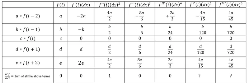
Since only the second derivative of the function is to be found out, the sum of the coefficients of `f’’(i) (dx)^2` alone equal to 1 and rest all are zero. Since we require only 5 equations to find the 5 coefficients, the last two columns are ignored for now.
Therefore considering the coefficients of the five columns ( `f(i)-f^(IV) (i) (dx)^4`), we have:
a+b+c+d+e = 0
-2a-b+d+2e = 0
4a/2+b/2+d/2+4e/2 =1
-8a/6-b/6+d/6+8e/6 = 0
2a/3+b/24+d/24+2e/3 =0
Converting the above equations, into matrix form:
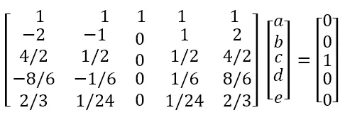
Solving the matrix by inversion leads to:
a =-0.08333333333333333333333333
b = 1.33333333333333333333333333
c =-2.50000000000000000000000000
d =1.333333333333333333333333333
e = -0.0833333333333333333333333
hence a= e , b=d
substituting these values in the taylor table leads to:
sum of column 2 = a+b+c+d+e =0
similarly ,
sum of coefficients of column 3 = -2a-b+d+2e = -2a-b+b+2a = 0
sum of coefficients of column 4 = 4a/2+b/2+d/2+4e/2= 4a/2+b/2+b/2+4a/2 =4a+b = 4(-0.0833)+1.3333= 1
sum of coefficients of column 5 = -8a/6-b/6+d/6+8e/6 = -8a/6-b/6+b/6+8a/6 = 0
sum of coefficients of column 6 = 2a/3+b/24+d/24+2e/3 = 2a/3+b/24+b/24+2a/3 = 0
sum of coefficients of column 7 = (-4a/15)+(-b/120)+(d/120)+(4e/15) =(-4a/15)+(-b/120)+(b/120)+(4a/15) =0
sum of coefficients of column 8 = (4a/45)+(b/720)+(d/720)+(4e/45) =(4a/45)+(b/720)+(b/720)+(4a/45) = 8a/45+b/360
rewriting equation (1) in terms of Taylor series expansion of individual terms by substituting the coefficient values of a,b,c,d,e leads to:
`(δ^2 f)/(δx)^2 ≅ a* f(i-2) +b*f(i-1) + c*f(i)+d*f(i+1) +e*f(i+2) = 0+0+1(f’’(i) (dx)^2)+0+0+((8a)/45+b/360)(f^(VI) (i) (dx)^6)`
Dividing both sides by `(dx)^2` and rewriting as:
`(δ^2 f)/(δx)^2 ≅ ( a* f(i-2) +b*f(i-1) + c*f(i)+d*f(i+1) +e*f(i+2))/(dx)^2 = f’’(i)+O(dx)^4`
Hence, the above equation represents the fourth order central difference approximation for `(δ^2 f)/(δx)^2` and the term `O(dx)^4` represents truncation error of fourth order. Therefore,
`(δ^2 f)/(δx)^2 ≅ ( a* f(i-2) +b*f(i-1) + c*f(i)+d*f(i+1) +e*f(i+2))/(dx)^2` .....(4)
Substituting the values a,b,c,d,e in above equation we can find the fourth order central difference approximation of second derivative of a function.
2. Skewed right-sided difference method:
The order of accuracy for the Skewed right-sided method is found as:
P = N - Q
Where,
P is The order of accuracy
N is the number of nodes in the stencil
Q is the order of derivative
Therefore the number of nodes to be considered for a fourth-order accurate approximation of a second-order derivative by Skewed right-sided method is given by:
4 = N-2
N = 6.
For a Skewed right-sided method, a function at a node can be evaluated by considering the information on the right side in the numerical stencil. Hence the numerical stencil of a function f(x) with fourth-order approximation with 6 nodes at a point ‘i’ can be represented as:

The hypothetical second order derivative of function f(x) at ‘i’ considering the fourth order right sided skewed difference approximation in terms of information from right side nodes be written as:
`(δ^2 f)/(δx^2) ≅ g* f(i) +h*f(i+1) + j*f(i+2)+k*f(i+3) +l*f(i+4) +m*f(i+5)` .......(5)
Let g* f(i) = g* f(i),
Let ‘dx’ be the discretization size then from Taylor series expansion of the second term h* f(i+1) gives,
`h*f(i+1)=h [[f(i)+(f’(i)(2dx))/1!+(f’’(i) (dx)^2)/2!+(f’’’(i) (dx)^3)/3!+(f^(IV) (i) (dx)^4)/4!+(f^V (i) (dx)^5)/5!+f^(VI )(i) (dx)^6)/6!+⋯]`
Simplifying the above equation,
`h*f(i+1)=h f(i)+hf’(i)dx+h/2 f’’(i) (dx)^2+h/6 f’’’(i) (dx)^3+h/24 f^(IV )(i) (dx)^4+h/120 f^V (i) (dx)^5+h/720 f^(VI) (i) (dx)^6+…`
Similarly taylor series expansion of the third term j* f(i+2) gives,
`j×f(i+2)=j f(i)+2jf’(i)dx+4j/2 f’’(i) (dx)^2+8j/6 f’’’(i) (dx)^3+16j/24 f^(IV )(i) (dx)^4+32j/120 f^V (i) (dx)^5+64/720 f^(VI )(i) (dx)^6+...`
Similarly taylor series expansion of the fourth term k* f(i+3) gives,
`k×f(i+3)=k f(i)+3kf’(i)dx+9k/2 f’’(i) (dx)^2+27k/6 f’’’(i) (dx)^3+81k/24 f^(IV) (i) (dx)^4+243k/120 f^V (i) (dx)^5+729k/720 f^(VI )(i) (dx)^6+....`
Similarly taylor series expansion of the fifth term l* f(i+4) gives,
`l×f(i+4)=l f(i)+4ef’(i)dx+16l/2 f’’(i) (dx)^2+64l/6 f’’’(i) (dx)^3+256l/24 f^(IV)_ (i) (dx)^4+1024l/120 f^V (i) (dx)^5+4096/720 f^(VI) (i) (dx)^6+...`
Similarly taylor series expansion of the sixth term m* f(i+5) gives,
`m×f(i+5)=mf(i)+5mf’(i)dx+25m/2 f’’(i) (dx)^2+125m/6 f’’’(i) (dx)^3+625m/24 f^(IV )(i) (dx)^4+3125m/120 f^V (i) (dx)^5+15625m/720 f^(VI )(i) (dx)^6+…`
All the above expansions can be represented in tabular form called Taylor’s table as shown below:
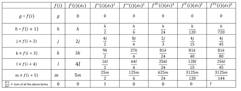
Since only the second derivative of the function is to be found out, the sum of the coefficients of `f’’(i) (dx)^2` alone equal to 1 and rest all are zero. Since we require only 6 equations to find the 6 coefficients, the last one columns is ignored for now.
Therefore considering the coefficients of the six columns ( `f(i)-f^(V) (i) (dx)^5`), we have:
g+h+j+k+l+m =0
h+2j+3k+4l+5m = 0
h/2 + 4j/2 +9k/2+16l/2+25m/2 = 1
h/6+8j/6+27k/6+64l/6+125m/6 =0
h/24+2j/3+81k/24+256l/24+625m/24=0
h/120+4j/15+81k/40+128l/15+3125m/120=0
Converting the above equations, into matrix form:
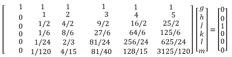
Solving the matrix by inversion leads to:
g = 3.750000000000000000000000
h = -12.8333333333333333333333
j = 17.83333333333333333333333
k = -13.00000000000000000000000
l = 5.083333333333333333333333
m = -0.83333333333333333333333
substituting these values in the taylor table leads to:
sum of column 2 coefficients = g+h+j+k+l+m = 0
sum of column 3 coefficients = h+2j+3k+4l+5m = 0
sum of column 4 coefficients = h/2 + 4j/2 +9k/2+16l/2+25m/2 = 1
sum of column 5 coefficients = h/6+8j/6+27k/6+64l/6+125m/6 = 0
sum of column 6 coefficients = h/24+2j/3+81k/24+256l/24+625m/24= 0
sum of column 7 coefficients = h/120+4j/15+81k/40+128l/15+3125m/120 = 0
sum of column 8 coefficients = h/720+4j/45+81k/80+256l/45+3125m/144 = non zero number
rewriting equation (5) in terms of Taylor series expansion of individual terms by substituting the coefficient values of g, h, j, k, l, m leads to:
`(δ^2 f)/(δx^2 ) ≅ g* f(i) +h*f(i+1) + j*f(i+2)+k*f(i+3) +l*f(i+4) +m*f(i+5) = 0+0+1(f’’(i) (dx)^2)+0+ 0+0+( h/720+4j/45+81k/80+256l/45+3125m/144)(f^(VI) (i) (dx)^6)+....`
Dividing both sides by `(dx)^2` and rewriting as,
`(δ^2 f)/(δx^2) ≅ (g* f(i) +h*f(i+1) + j*f(i+2)+k*f(i+3) +l*f(i+4) +m*f(i+5) )/(dx)^2 = f’’(i)+O(dx)^4`
Hence, the above equation represents the fourth order skewed right sided difference approximation for `(δ^2 f)/(δx)^2` and the term `O(dx)^4` represents truncation error of fourth order. Therefore,
`(δ^2 f)/(δx^2) ≅ ( g* f(i) +h*f(i+1) + j*f(i+2)+k*f(i+3) +l*f(i+4) +m*f(i+5))/(dx)^2` ....(6)
3. Skewed left-sided difference method:
The order of accuracy for the Skewed left sided method is found as:
P = N - Q
Where,
P is The order of accuracy
N is the Number of nodes in the stencil
Q is the order of derivative
Therefore the number of nodes to be considered for a fourth order accurate approximation of a second order derivative by Skewed left sided method is given by:
4 = N-2
N = 6.
For a Skewed left-sided method, a function at a node can be evaluated by considering the information on the left side in the numerical stencil. Hence the numerical stencil of a function f(x) with fourth-order approximation with 6 nodes at point ‘i’ can be represented as:

The hypothetical second order derivative of function f(x) at ‘i’ considering the fourth order left sided skewed difference approximation in terms of information from left side nodes be written as:
`(δ^2 f)/(δx^2) ≅ n* f(i-5) +p*f(i-4) + q*f(i-3)+r*f(i-2) +s*f(i-1) +t*f(i)` ....(7)
Let t* f(i) = t* f(i),
Let ‘dx’ be the discretization size then from Taylor series expansion of the first term n* f(i-5) gives,
`n*f(i-5)=n [f(i)-(f’(i)(5dx))/1!+(f’’(i) (5dx)^2)/2!-(f’’’(i) (5dx)^3)/3!+(f^(IV) (i) (5dx)^4)/4!-(f^V (i) (5dx)^5)/5!+(f^(VI) (i) (5dx)^6)/6!+⋯]`
Simplifying the above equation,
`n*f(i-5)=n f(i)-5nf’(i)dx+25n/2 f’’(i) (dx)^2-125n/6 f’’’(i) (dx)^3+625n/24 f^(IV )(i) (dx)^4-3125n/120 f^V (i) (dx)^5+15265n/720 f^(VI) (i) (dx)^6+…`
Similarly taylor series expansion of the second term p*f(i-4) gives,
`p×f(i-4)=l f(i)-4pf’(i)dx+16p/2 f’’(i) (dx)^2-64p/6 f’’’(i) (dx)^3+256p/24 f^(IV )(i) (dx)^4-1024p/120 f^V (i) (dx)^5+4096/720 f^(VI )(i) (dx)^6+...`
Similarly taylor series expansion of the third term q*f(i-3) gives,
`q×f(i-3)=k f(i)-3qf’(i)dx+9q/2 f’’(i) (dx)^2-27q/6 f’’’(i) (dx)^3+81q/24 f^(IV) (i) (dx)^4-243q/120 f^V (i) (dx)^5+729q/720 f^(VI) (i) (dx)^6+…`
Similarly taylor series expansion of the fourth term r* f(i-1) gives,
`r*f(i-2)=r f(i)-2rf’(i)dx+4r/2 f’’(i) (dx)^2-8r/6 f’’’(i) (dx)^3+16r/24 f^(IV )(i) (dx)^4-32r/120 f^V (i) (dx)^5+64r/720 f^(VI )(i) (dx)^6+…`
Similarly taylor series expansion of the fifth term s* f(i-1) gives,
+…`s*f(i-1)=s f(i)-sf’(i)dx+s/2 f’’(i) (dx)^2-s/6 f’’’(i) (dx)^3+s/24 f^(IV) (i) (dx)^4-s/120 f^V (i) (dx)^5+s/720 f^(VI) (i) (dx)^6+…`
All the above expansions can be represented in tabular form called Taylor’s table as shown below:
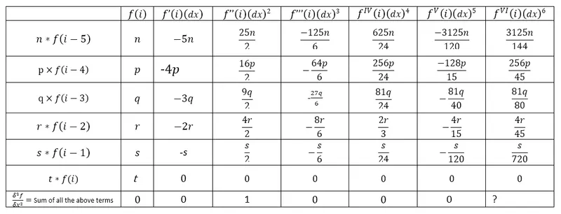
Since only the second derivative of the function is to be found out, the sum of the coefficients of `f’’(i) (dx)^2` alone equal to 1 and rest all are zero. Since we require only 6 equations to find the 6 coefficients, the last one columns is ignored for now.
Therefore considering the coefficients of the six columns ( `f(i)-f^(V) (i) (dx)^5`), we have:
n+p+q+r+s+t =0
-5n-4p-3q-2r-s = 0
25n/2+16p/2+9q/2+4r/2+s/2 = 1
-125n/6-64p/6-27q/6-8r/6-s/6=0
625n/24+256p/24+81q/24+2r/3+s/24 =0
-3125n/120-128p/15-81q/40-4r/15-s/120=0
Converting the above equations, into matrix form:

Solving the matrix by inversion leads to:
n = -0.833333333333333333333333
p = 5.0833333333333333333333333
q = -13.00000000000000000000000
r = 17.833333333333333333333333
s = -12.83333333333333333333333
t = 3.7500000000000000000000000
substituting these values in the taylor table leads to:
sum of column 2 coefficients = n+p+q+r+s+t = 0
sum of column 3 coefficients = -5n-4p-3q-2r-s = 0
sum of column 4 coefficients = 25n/2+16p/2+9q/2+4r/2+s/2 = 1
sum of column 5 coefficients = -125n/6-64p/6-27q/6-8r/6-s/6=0
sum of column 6 coefficients = 625n/24+256p/24+81q/24+2r/3+s/24 =0
sum of column 7 coefficients = -3125n/120-128p/15-81q/40-4r/15-s/120=0
sum of column 8 coefficients = 3125n/144+256p/45+81q/80+4r/45+s/720=non zero number
rewriting equation (5) in terms of Taylor series expansion of individual terms by substituting the coefficient values of n,p,q,r,s,t leads to:
`(δ^2 f)/(δx^2) ≅ n* f(i-5) +p*f(i-4) + q*f(i-3)+r*f(i-2) +s*f(i-1) +t*f(i) = 0+0+1(f’’(i) (dx)^2)+0+ 0+0+( 3125n/144+256p/45+81q/80+4r/45+s/720)(f^(VI) (i) (dx)^6)+...`
Dividing both sides by `(dx)^2` and rewriting as
`(δ^2 f)/(δx^2) ≅ (n* f(i-5) +p*f(i-4) + q*f(i-3)+r*f(i-2) +s*f(i-1) +t*f(i))/(dx)^2 = f’’(i)+O(dx)^4`
Hence, the above equation represents the fourth order skewed left sided difference approximation for `(δ^2 f)/(δx)^2` and the term `O(dx)^4` represents truncation error of fourth order. Therefore,
`(δ^2 f)/(δx^2) ≅ ( n* f(i-5) +p*f(i-4) + q*f(i-3)+r*f(i-2) +s*f(i-1) +t*f(i))/(dx)^2` ......(8)
II. Objectives:
- To write a program in Matlab to evaluate the second-order derivative of the function exp(x)*cos(x) and compare the errors of the 3 numerical approximations derived for fourth-order accuracy.
- Plot the graph that compares the error for the numerical schemes derived.
III. Program:
The main program code is given below:
%program that compares the first, second and fourth order approximations of the second derivative against the analytical or exact derivative for f(x) = exp(x)*cos(x).

clear all
close all
clc

%Input analytical function
%f(x) = exp(x)*cos(x);

%input value of x
x = pi/3;

%dicretization size in x
dx = linspace(pi/4000,pi/40,20);

%Error in numerical approximations values over the entire dx range computed by calling the appropriate function handles
for i = 1:length(dx)
E_FCDA(i) = numerical_function(x,dx(i));        %fourth order central difference approximation error
E_FSRA(i) = numerical_function1(x,dx(i));        %fourth order skewed right sided difference approximation error
E_FSLA(i) = numerical_function2(x,dx(i));         %fourth order skewed left sided approximation error
end

%loglog plot of errors vs dx
figure(1)
loglog(dx,E_FSRA,'b-*')
hold on
loglog(dx,E_FSLA,'g-*')
loglog(dx,E_FCDA,'r-*')
xlabel('discretization size (dx)')
ylabel('Error in approximation')
legend('Error FSRA','Error FSLA','Error FCDA')
title('Error for different approximation schemes')
Code Explanation:
Step1: clear all – command to clear the workspace.
Step 2: close all – command to close all opened previous plots.
Step 3: clc – command to clear the command window.
Step 4: Define the input value of 'x =pi/3' to be solved for the function.
Step 5: defining the discretization range as array 'dx =(pi/4000,pi/40,20)'.
Step 6: computing the numerical approximation error value of the second derivative of the given function by calling a function code 'numerical_function' , 'numerical_function1' and 'numerical_fucction2' for fourth-order accurate centered, right-skewed, and left-skewed difference methods in a for loop to index over the entire range of dx. The function codes are given below:
Function code for fourth_order_central_difference_approximation:
function [E_FCDA] = numerical_function(x,dx)

%analytical/exact second  deraivative
AFD = -2*exp(x)*sin(x);

%numerical approximations of second deriavative of a function

%fourth_order_central_difference_approximation

%f''(x) = ((a* f(i-2) +b*f(i-1) + c*f(i)+d*f(i+1) +e*f(i+2))/(dx)^2
%a,b,c,d,e are coefficients of approximation by taylor's table method
a =-0.08333333333333333333333333
b = 1.33333333333333333333333333
c =-2.50000000000000000000000000
d =1.333333333333333333333333333
e = -0.0833333333333333333333333

FCDA = (a*exp(x-2*dx)*cos(x-2*dx)+b*exp(x-dx)*cos(x-dx)+c*exp(x)*cos(x)+d*exp(x+dx)*cos(x+dx)+e*exp(x+2*dx)*cos(x+2*dx))/(dx^2)

%Errors in fourth order central difference approximation
E_FCDA = abs(FCDA-AFD);

end
Function code for fourth_order_skewed right sided _difference_approximation:
function [E_FSRA] =  numerical_function1(x,dx)

%analytical/exact second  deraivative
AFD = -2*exp(x)*sin(x);

%numerical approximations of second deriavative of a function
%fourth_order skewed right sided _approximation
%f''(x) = ((g* f(i)) +(h*f(i+1)) + (j*f(i+2))+k*f(i+3) +l*f(i+4)+m*f(i+5))/(dx)^2

%g,h,j,k,l,m are coefficients of approximation by taylor's table method
  g =  3.750000000000000000000000
  h =  -12.8333333333333333333333
  j =  17.83333333333333333333333
  k = -13.00000000000000000000000
  l =  5.083333333333333333333333
  m =  -0.83333333333333333333333


FSRA = ((g*(exp(x)*cos(x)))+(h*(exp(x+dx)*cos(x+dx)))+(j*(exp(x+2*dx)*cos(x+2*dx)))+(k*(exp(x+3*dx)*cos(x+3*dx)))+(l*(exp(x+4*dx)*cos(x+4*dx)))+(m*(exp(x+5*dx)*cos(x+5*dx))))/(dx)^2

%Errors in FRSA approximation
E_FSRA = abs(FSRA-AFD);


end
Function code for fourth_order_skewed left sided _difference_approximation:
function [E_FSLA] =  numerical_function2(x,dx)

%analytical/exact second  deraivative
AFD = -2*exp(x)*sin(x);
%fourth_order  skewed left sided_approximation
%f''(x) = ((n* f(i-5)) +(p*f(i-4)) + (q*f(i-3))+r*f(i-2) +s*f(i-1)+t*f(i))/(dx)^2

%n,p,q,r,s,t are coefficients of approximation by taylor's table method
 n = -0.833333333333333333333333
 p = 5.0833333333333333333333333
 q = -13.00000000000000000000000
 r = 17.833333333333333333333333
 s = -12.83333333333333333333333
 t = 3.7500000000000000000000000

FSLA = ((n*(exp(x-5*dx)*cos(x-5*dx)))+(p*(exp(x-4*dx)*cos(x-4*dx)))+(q*(exp(x-3*dx)*cos(x-3*dx)))+(r*(exp(x-2*dx)*cos(x-2*dx)))+(s*(exp(x-1*dx)*cos(x-1*dx)))+(t*(exp(x)*cos(x))))/(dx)^2

%Errors in FRSA approximation
E_FSLA = abs(FSLA-AFD);
end
The function codes take x and dx as input arguments and output the error in approximation with respect to the analytical/exact second deraivative of the function 'f(x) = exp(x)*cos(x)'
The numerical approximations are found using the derived equations and coefficients from the Taylor's table method.
These function codes are called in the main program to calculate the errors for the entire range of dx using for loop.
step 7: plotting the error in approximations in the log-log plot.
IV Output:
The output of the program is the comparison of error values of different approximation schemes for the second derivative of function exp(x)*cos(x) using fourth-order central difference, right-skewed difference and left-skewed difference methods with respect to exact derivative. The comparison is shown in the plot shown below:
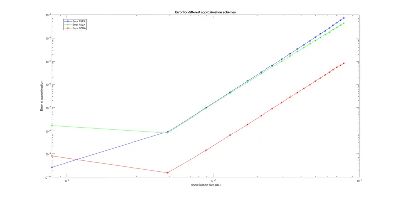
It can be seen from the above plot, the central difference scheme has the lowest error when compared to the right and left-skewed difference methods. Also, the error values decrease rapidly as the discretization size decreases up to some extent and thereafter, the error starts increasing. This change in the trend of the error is due to the round off error occurring due to computational limits. Hence while choosing the discretization size, care should be taken to account for round off errors due to computational limits.
Although the central difference method has the lowest error values when compared to skewed method, skewed methods are more useful because we can predict the derivative of a function at a point by knowing the values of the function only on one side of the point (left or right). This is of greater benefit when we have information about the function on only one side of the point in the numerical stencil. Whereas, the central difference method requires information on both sides of the point in the numerical stencil.
References: