Optimizing the stalagmite function using Genetic Algorithm in MATLAB
I. Aim: The aim of this project is to optimize a stalagmite function and find the global maxima using a genetic algorithm in MATLAB.
Introduction:
A. Stalagmite function:
A stalagmite function is a mathematical model representing the maxima and minimum of a function z= f(x,y) as a surface with stalagmite rock-like structures to represent the maxima of ‘z’ in terms of x and y. The equations for the stalagmite function ‘z’ are represented mathematically as:
`z(x,y)=z_(1x)×z_(2x)×z_(1y)×z_(2y)` ;
`z_(1x)=[sin(5.1πx+0.5)]^6`;
`z_(1y)=[sin(5.1πy+0.5)]^6`;
`z_(2x)=exp[-4ln(2)×(x-0.0667)^2/0.64]`;
`z_(2y)=exp[-4ln(2)×(y-0.0667)^2/0.64]`;
A general stalagmite function is shown in the below figure:
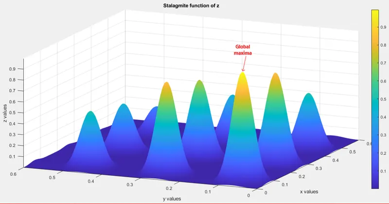
The surface consists of minima and maxima of a function. The peaks of stalagmite like structures represent the local maxima’s and the highest of them represents the global maxima of the function as shown in the above figure. Finding the global maxima or minima of a function(z) is more of an optimization technique and becomes tedious when the data of input variables(x,y) is vast. So, we use an algorithm to optimize the stalagmite function and find the global maxima.
B. Optimization:
It is a decision-making technique used to find the best set of solutions for a particular problem under certain predefined constraints. It is an iterative process of comparing various solutions until an optimum solution or satisfactory solution is found. It can be maximizing/minimizing a function, maximizing productivity, reducing the cost, increasing durability etc. For this, appropriate algorithms are used depending on the type of problem.
C. Genetic Algorithm:
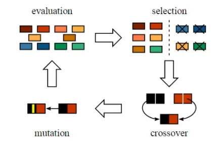
Genetic Algorithms (GAs) are adaptive heuristic search algorithms and are part of evolutionary algorithms. Genetic algorithms are based on Darwin’s theory of evolution which is the idea of natural selection and genetics. To generate high-quality solutions for optimization problems and search problems genetic algorithms are widely used.
For optimizing a problem genetic algorithm, simulate the process of natural selection between individuals (survival of the fittest). The species which can adapt to changes in their environment are able to survive and reproduce and go to the next generation. Each and every individual represents a point in search space and possible solution and a population of individuals constitutes a generation. Each individual is represented as a string of character/integer/float/bits. This string is analogous to the chromosome in genetic theory.
The flowchart for a general genetic algorithm is given below:
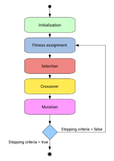
Steps involved in Genetic Algorithm:
1. Initialisation:
The genetic algorithm starts with the initialisation of the population that is selected as the search space for finding the optimum solution. The population is the number of data points selected to perform the genetic algorithm.
2. Selection:
In this step possible fittest individuals from the population are selected that can reproduce better offsprings and are designated as parents. But this will lead to offsprings of similar characteristics and little diversity. Hence, a roulette wheel type selection method is employed.
The roulette wheel is divided that into m divisions(pie), where m is the number of individuals in our populations. The area occupied by each individual will be proportional to its fitness value. Fitness value represents how fit it is to produce better offsprings.
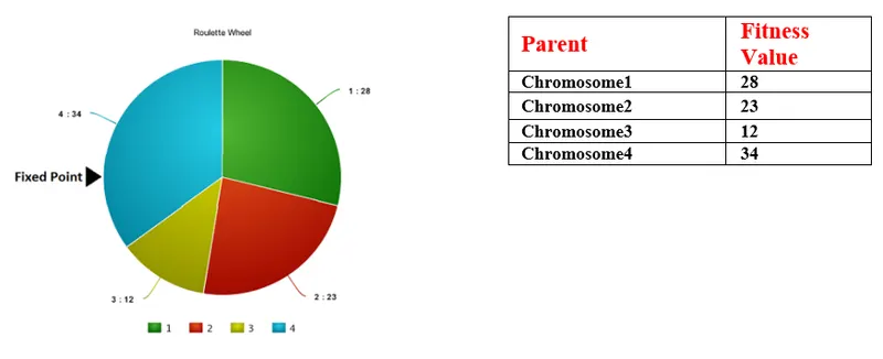
The wheel is also marked with a fixed point. The wheel is rotated and every time it stops on a particular pie, that individual is selected as the parent. This step is repeated and a number of parents are selected. The idea of using greater pie for fitter individual is that the chance of these getting selected as parents is high. Sometimes two marks are also used, such that we can get both the parents in one go. This method is known as the Stochastic Universal Selection method.
3. Crossover:
It is the process of producing offspring from two selected parents. There are different methods of cross-over. A one-point crossover method is explained below:
Consider chromosome1 and chromosome4, which are the fittest in the group as selected parents. An offspring is produced by the crossover of a random set of genes of chromosome1 and chromosome4 as shown below. Here, the tails of the parents are joined to produce the new offspring.
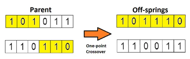
0 and 1 represent the genes of the chromosomes.
4. Mutation:
In order to have diversity in the new generation, mutation is carried out after the crossover. It is the idea of tweaking the new chromosome to have more diversity in the population.
This is essential to keep the offsprings having characteristics different from their parents and to maintain genetic diversity from generation to others. They are different methods of mutation and one such method is shown below:

In the above example, a gene (1) in the third-place of the offspring chromosome is replaced with a new gene (0) to have different characteristics.
The above processes of selection, crossover, the mutation for the offspring are repeated by replacing the parents until an optimized solution is found.
The entire process can be summarised as below:
D. Fitness function:
It is a function that evaluates how close the possible solution is to the optimum solution for the problem. It takes the solution as the input and produces the suitability of the solution output. The off-springs thus produced are validated using the fitness function, and if considered fit then will replace the less fit chromosomes from the population.
But there should be a limit for the algorithm iterations to check when we can attain an optimum solution. This can be realized using termination conditions for the algorithm and are as follows:
- When there is no improvement in the population after x iterations (generations).
- A predefined absolute number of generations for our algorithm is reached.
- When the fitness function (objective function) has reached a predefined value.
MATLAB has an inbuilt optimization genetic algorithm ‘ga’ to find global minima for a function. In order to find the global maxima of the stalagmite function using ‘ga’, modification has to be done in the objective function of stalagmite.
II. Objectives:
- Write a code in MATLAB to optimise the stalagmite function and find the global maxima of the function.
- Check the convergence of the 'ga' for the global maxima of the stalagmite function.
III. Program:
The program for optimizing the stalagmite function and finding global maxima using ‘ga’ is given in the code below:
clear all
close all
clc


%defining the search space
x = linspace(0,0.6,150);
y = linspace(0,0.6,150);
num_cases= 50;             %number of iterations used by ga


%meshgrid to create 2d array
[xx yy] = meshgrid(x,y);

for i=1:length(xx)
    for j=1:length(yy)
        input_vector(1)=xx(i,j);
        input_vector(2)=yy(i,j);
        F(i,j) = stalagmite(input_vector);      %creating the stalagmite matrix using stalgmite function and input variables xx,yy over the length of xx, yy vector
    end
end

%study 1 random sampling
tic                         %tic-toc command to count the time taken for the excecution
for n = 1:num_cases         % iterating n times the GA function to find the global maxima

[inputs, Fopt(n)] = ga(@stalagmite, 2);         % syntax to get the optimum value of stalagmite and its input variables using GA
xopt(n) = inputs(1);
yopt(n) = inputs(2);
end
solve_time1 = toc

%plotting the stalagmite function and the maximum in the same same figure
figure(1)
subplot(2,1,1)                  %syntax for plotting multiple plots in same figure, plot in the figure1 at 1st row of 2 rows,1 column of total 1 column and at 1st element
surfc(x,y,-F)                     %plot of stalagmite function in terms of x,y and since F=-f
hold on
xlabel ('x values')
ylabel ('y values')
zlabel('f values')
shading interp                                      %to hide the meshlines on the plot
title('f maximum with no upper and lower bounds','50 iterations')
colorbar
plot3(xopt,yopt,-Fopt,'r-o','markerfacecolor','r') %plot of optimum F, x,y predicted by ga

subplot(2,1,2)              %plot in the figure1 at 2nd row of 2 rows,1 column of total 1 column and at second element
plot(-Fopt, 'linewidth',2)
xlabel('iterations')
ylabel('f maximum')
title('f maximum vs no. of iterations')

%study 2 sampling with lower and upper bounds for input variables
tic
for m = 1:num_cases

[inputs, Fopt(m)] = ga(@stalagmite, 2,[],[],[],[],[0;0],[0.6;0.6]); %defines a set of lower and upper bounds on the design variables,[inputs, Fopt(m)], so that a solution is found in the range [0;0] to [0.6;0.6]. syntax for setting the upper and lower bounds for input variables of the GA search space
xopt(m) = inputs(1);
yopt(m) = inputs(2);
end
solve_time2 = toc
figure(2)
subplot(2,1,1)
surfc(x,y,-F)
hold on
xlabel ('x values')
ylabel ('y values')
zlabel('f values')
title('f maximum with upper and lower bounds','50 iterations')
shading interp
colorbar
plot3(xopt,yopt,-Fopt,'r-o','markerfacecolor','r')

subplot(2,1,2)
plot(-Fopt, 'linewidth',2)
xlabel('iterations')
ylabel('f maximum')
title('f maximum vs no. of iterations')

%Increasing the population size to 180
options = optimoptions('ga');                           %syntax to return a set of default options for the 'ga' solver.
options = optimoptions(options,'PopulationSize',180);   %syntax that returns a copy of options with the populationsize altered with the value 180 for the 'ga' solver.

%Study 3 for 50 iterations and population size 180
tic
for l = 1:num_cases

[inputs, Fopt(l)] = ga(@stalagmite, 2,[],[],[],[],[0;0],[0.6;0.6],[],[],options);  %minimizes with the default optimization parameters replaced by values in options (syntax for finding the optimum value(maxima) of the stalagmite function using ga algorithm for the adjusted polulation size 180)
xopt(l) = inputs(1);
yopt(l) = inputs(2);
end
solve_time3 = toc
figure(3)
subplot(2,1,1)
surfc(x,y,-F)
hold on
xlabel ('x values')
ylabel ('y values')
zlabel('f values')
title('f maximum with upper and lower bounds', 'population size 180 and 50 iterations')
shading interp
colorbar
plot3(xopt,yopt,-Fopt,'r-o','markerfacecolor','r')

subplot(2,1,2)
plot(-Fopt, 'linewidth',2)
xlabel('iterations')
ylabel('f maximum')
title('f maximum vs no. of iterations')

%keeping the population size of 180
options = optimoptions('ga');
options = optimoptions(options,'PopulationSize',180);
%Study 4 for 70 iterations and population size 180
tic
for l = 1:70

[inputs, Fopt(l)] = ga(@stalagmite, 2,[],[],[],[],[0;0],[0.6;0.6],[],[],options);
xopt(l) = inputs(1);
yopt(l) = inputs(2);
end
solve_time4 = toc
figure(4)
subplot(2,1,1)
surfc(x,y,-F)
hold on
xlabel ('x values')
ylabel ('y values')
zlabel('f values')
title('f maximum with upper and lower bounds','population size 180 and 70 iterations')
shading interp
colorbar
plot3(xopt,yopt,-Fopt,'r-o','markerfacecolor','r')

subplot(2,1,2)
plot(-Fopt, 'linewidth',2)
xlabel('iterations')
ylabel('f maximum')
title('f maximum vs no. of iterations')

%keeping the population size of 180
options = optimoptions('ga');
options = optimoptions(options,'PopulationSize',180);
%Study 5 for 80 iterations and population size 180
tic
for l = 1:80

[inputs, Fopt(l)] = ga(@stalagmite, 2,[],[],[],[],[0;0],[0.6;0.6],[],[],options);
xopt(l) = inputs(1);
yopt(l) = inputs(2);
end
solve_time5 = toc
figure(5)
subplot(2,1,1)
surfc(x,y,-F)
hold on
xlabel ('x values')
ylabel ('y values')
zlabel('f values')
title('f maximum with upper and lower bounds','population size 180 and 80 iterations')
shading interp
colorbar
plot3(xopt,yopt,-Fopt,'r-o','markerfacecolor','r')

subplot(2,1,2)
plot(-Fopt, 'linewidth',2)
xlabel('iterations')
ylabel('f maximum')
title('f maximum vs no. of iterations')
Code Explanation:
Step1: clear all – command to clear the workspace.
Step 2: close all – command to close all opened previous plots.
Step 3: clc – command to clear the command window.
Step 4:
The next step is to define the input variables (x,y) for the stalagmite function F. These are input as arrays. A variable num_cases is created to store the number of iterations for the ‘ga’ algorithm.
meshgrid command is used to create 2d arrays from the 1d arrays of x and y.
These are used as input vector variables for the stalagmite function. The stalagmite function code is as shown below:
function [F] = stalagmite(input_vector)

f_1x = (sin((5.1*pi*input_vector(1))+0.5)).^6;
f_1y = (sin((5.1*pi*input_vector(2))+0.5)).^6;
f_2x = exp(-4*log(2)*((input_vector(1)-0.0667).^2/0.64));
f_2y = exp(-4*log(2)*((input_vector(2)-0.0667).^2/0.64));
f = (f_1x.*f_2x.*f_1y.*f_2y);                   %stalagmite function formula
F=-f;                       % ga in matlab finds only mimima of a fuction, so to obtain the maxima value using ga we should make the function as negative

end
Function code explanation:
The function ‘stalagmite outputs an argument ‘F’ which represent the stalagmite surface dependent on xx and yy input vectors. The equation for finding the stalagmite function discussed in the introduction section is coded in this function handle. The function has only one input argument because ‘ga’ supports only one input argument at a time. The term ‘F=-f’ is used because ‘ga’ finds only the minima of a function. To find the maxima(peak value) of the stalagmite function, it is multiplied by -1.
Step 5:
The output of the stalagmite function is iterated over the length of xx vector and yy vector to get the corresponding F matrix values using nested for loop commands.
Step 6:
In this step, the stalagmite function is optimized to find the optimum F value and corresponding x and y values using the ‘ga’ algorithm. The syntax for the same is :
[inputs, Fopt(n)] = ga(@stalagmite, 2);
Where inputs and Fopt are the output arguments from the ‘ga’ algorithm. @stalagmite is the objective function and the number of design variables is 2 (x,y). The ‘ga’ is run for 50 iterations for random sampling using a for loop. Also, the time for the iterations is counted using the tic-toc command.
Step 7:
The stalagmite surface ('f = -F' in terms of x,y) and the optimum F,x,y , the output from the above ‘ga’ code execution are plotted in the first subplot and optimum stalagmite value (maxima) 'f =-F' variation with respect to iterations in the second subplot in a single figure using the subplot command.
Step 8:
The above process is repeated in this step with keeping bounds on the input variables x,y for ‘ga’. This is to limit the ‘ga’ for searching for optimum values outside the input variable range.
The syntax for the same is:
[inputs, Fopt(m)] = ga(@stalagmite, 2,[],[],[],[],[0;0],[0.6;0.6])
The blank parentheses [],[],[],[],[] represent that there are no linear exist in the function. The parentheses [0;0],[0.6;0.6] are the upper and lower bounds of design variables x,y and this limits the search space of ‘ga’.
Once optimum F,x,y are found from this bounded ‘ga’, the results are plotted similarly to the previous step.
Step 9:
In this step the population size of the ‘ga’ search space is increased to 180 from random point selection. The syntax for setting population size is:
options = optimoptions('ga');
this syntax returns a set of default options for the ‘ga’ solver.
options = optimoptions(options,'PopulationSize',180);
this syntax returns options with the population size altered with the specified value 180.
Step10:
In this step the stalagmite function is optimized to find the optimum F value and corresponding x and y values using the ‘ga’ algorithm for the new population size of 180. The syntax for the same is :
[inputs, Fopt(n)] = ga(@stalagmite, 2 ,[],[],[],[],[0;0],[0.6;0.6],[],[],options);
Where, options in the syntax represents the population size. The ‘ga’ is run for 50 iterations for using a forloop within the upper and lower bounds of design variables x,y [0;0],[0.6;0.6] . plotting is similar to above steps.
Step 11:
To check for convergence in the optimum F,x,y values the ‘ga’ algorithm with upper and lower bounds of design variables x,y and population size 180 is iterated for 70 and 80 iterations in the next sections of the code and plotting is done similarly to the sections above.
IV. Errors:
- While excecuting the function code an error was thrown in the command window as shown below:
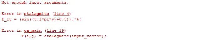
This error was due to giving input arguments as x,y for the stalagmite function and calling the function with input_vector as input argument in the main ‘ga’ code.
It is rectified by changing the input arguments of stalagmite function as:
function [F] = stalagmite(input_vector)
2. Unrecognised function or variable optimoption.
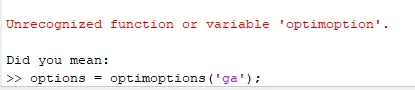
The error is due to a typo error in syntax for the option command of ‘ga’.
It is rectified by correcting the syntax as:
options = optimoptions('ga');
V. Output:
A Matlab code is written to optimize and find the global maxima of the stalagmite function using the ‘ga’ genetic algorithm. Since ‘ga’ only minimizes a function, the stalagmite function is modified (f =-F) to obtain maxima from the ‘ga’ algorithm in Matlab. A total of 5 cases were studied to optimize and to analyse the effect of population size and iterations(generations) effect on the global maxima of the stalagmite function.
Case1: Random sampling with 50 iterations
In this case, the ‘ga’ is allowed to take data points randomly with no bound on the design variables. The iteration limit is set to 50 iterations, to avoid the algorithm running for long durations. The maxima(optimum f value) predicted by the ‘ga’ for random sampling and 50 iterations is shown in the below figure:
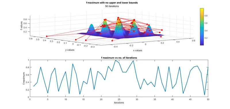
The ‘ga’ predicted the optimum value to be at different data points(x,y). These are the local maxima of ‘f’ but not the global maxima. Also, the search space was not limited to the x,y limits since the ‘ga’ randomly selected the search for the 50 iterations.
Case 2: Sampling with upper and lower bounds on design variables.
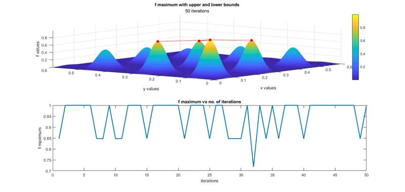
To better optimize the function and get the global maxima by limiting the search space within the bounds of design variables, this case is run by limiting the search space of ‘ga’ within the bounds of design variables(x,y) limits. The iteration limit is the same as case 1. The predicted maxima points are within the input design variables limit with a much more optimised range of f value. The maxima were found to be at the four highest peaks of the function indicated by the red line and dots in the below plot. These points represent the local maxima around those peaks. Still, this function can be optimised to find global maxima. From the iteration plot, it can be inferred that the maxima values are between 0.7 to 1.
Case 3: Population size of 180 and 50 iterations.
To get a more optimised solution, the number of data points (population size) is increased to 180 and 50 iterations are carried with upper and lower bounds for design variables. This resulted in a much more optimised value for the maxima as shown in the below plot.
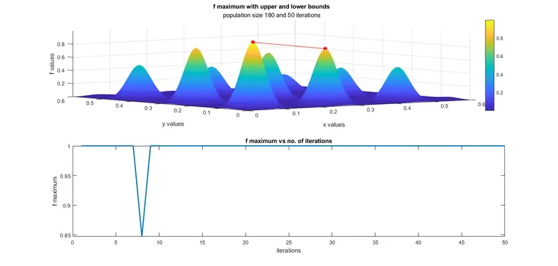
The optimum f value(maxima) is falling at the two peaks and has the value of 1 throughout the 50 iterations except for the 8th iteration, where the value is 0.85. Hence increasing the population size greatly optimised the function.
Case 4: Population size of 180 and 70 iterations.
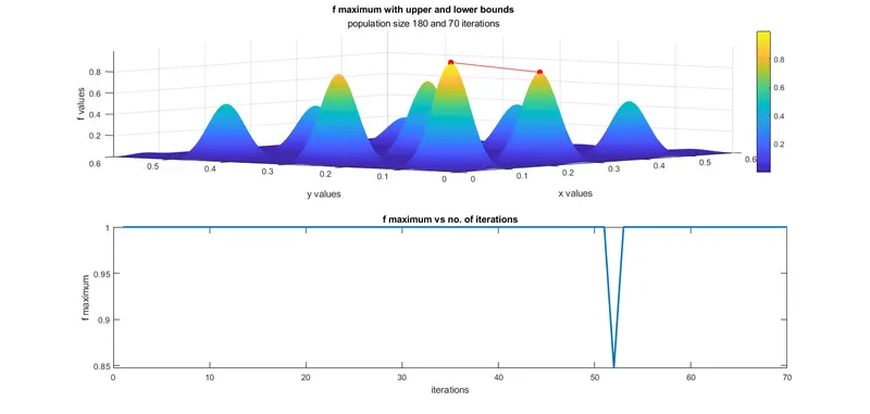
This case is similar to case 3, except for an increase in iterations from 50 to 70. As the solution from the previous case is nearer to the optimum value, the effect of iterations on the result is evaluated in this case. The results were similar to case 3 with the optimum f value being 1throughout the iterations except for the 52nd iteration with a value of 0.85.
Case 5: Population size of 180 and 80 iterations.
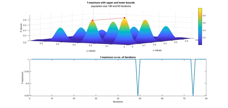
This case is similar to case 3, except for an increase in iterations from 50 to 80. As, the solution from the previous case is nearer to the optimum value, the effect of iterations on the result is evaluated in this case. In this case, the results were similar to case 3 with the optimum f value being 1 throughout the iterations except for 49th and 74th iterations with a value of 0.85.
This indicates that the ‘ga’ algorithm converged to an optimum solution (global maxima) for the stalagmite function. The value is f_opt= -F_opt=1.
The design variables at which the stalagmite function has a global maximum of f_opt= 1, are x = 0.0668 and y = 0.0668, which are confirmed from the output of the ‘ga’ algorithm as shown below:



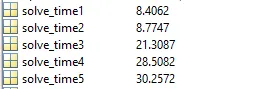
Although, increasing the iterations and population size optimises the solution of ‘ga’, the time for executing the ‘ga’ increases. The time for each case is given in the following image:
VI. Conclusion:
Genetic algorithms can be used to optimize a particular function. These are based on the theory of natural selection and genetics. In this project, a Matlab code is executed to optimize the stalagmite function using a genetic algorithm. The global maxima of the stalagmite function is found by optimising the stalagmite function by using the ‘ga’ algorithm. The solution predicted by a ‘ga’ algorithm can be optimised by proper selection of population size, search space and number of iterations.
References:
- https://skill-lync.com/knowledgebase/genetic-algorithm-explained
- https://www.analyticsvidhya.com/blog/2017/07/introduction-to-genetic-algorithm/
- https://www.geeksforgeeks.org/genetic-algorithms/
- http://www.jade-cheng.com/au/coalhmm/optimization/
- https://www.neuraldesigner.com/blog/genetic_algorithms_for_feature_selection
- https://in.mathworks.com/matlabcentral/answers/52240-how-to-find-max-fuction-with-genetic-algorithm
- https://in.mathworks.com/help/gads/how-the-genetic-algorithm-works.html
- https://in.mathworks.com/help/gads/ga.html
- https://towardsdatascience.com/introduction-to-genetic-algorithms-including-example-code-e396e98d8bf3