Week 4.1 - Linear Convection for varying number of nodes

QUESTION:

Numerical solution to the One-dimensional Linear Convection equation.

1. Assume that the domain length is L = 1m
2. The initial velocity profile is a step function. It is equal to 2m/s between x= 0.1 and 0.3 and 1m/s everywhere else
3. Use first-order forward differencing for the time derivative
4. Use first-order backward/rearward differencing for the space term.
5. Constant convection coefficient, c = 1 m/s
6. Time step, dt = 0.01
7. Simulation run time, t = 0.4 seconds.

Perform the simulation for the Number of nodes, n=20,40,80 and 160.

EXPECTED OUTPUT:

1. Compare the original and final velocity profiles in a single figure window.
2. You will get 4 plots in total, one for each n, and you will upload the plots in the challenge space provided using the Insert/edit image option.
3. From the plots obtained: Explain in detail the phenomena observed- numerical diffusion and instability and how they relate to the courant number and the accuracy of the solution. How does a change in grid size affect these phenomena?

ANSWER:

AIM:

• To obtain a numerical solution to the one-dimensional linear convection equation and perform simulation for the number of nodes n = 20, 40, 80, 160.
• To explain the phenomena observed – numerical solution and instability and how they are related to courant number and the accuracy of the solution.
• To explain how those changes in grid size affect this phenomenon.

Assumption and input:

• Assume that the domain length is L = 1m
• The initial velocity profile is a step function. It is equal to 2m/s between x= 0.1 and 0.3 and 1m/s everywhere else.
• Use first-order forward differencing for the time derivative.
• Use first-order backward/rearward differencing for the space term.
• Constant convection coefficient, c = 1 m/s
• Time step, dt = 0.01
• Simulation run time , t = 0.4 seconds.
• Perform the simulation for the Number of nodes, n=20,40,80 and 160.

Solution:

The one-dimension linear convection equation is written as,

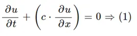
Where u = Velocity and c = Convective coefficient.

Given that we have to use first-order forward differencing for the time derivative term and first-order backward differencing for space term.

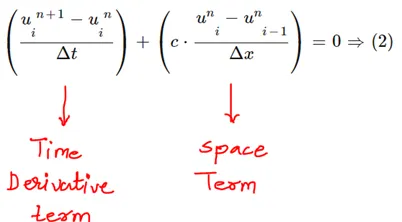
Rewriting the above equation, we get,

The above equation is used in MATLAB code to obtain a solution.

INPUTS:

[MATLAB CODE]

Following MATLAB code is for 20 grid points.

Similar in been done for the grid points 40, 80, and 160.

%% Clearing
clc
clear all
close all

%% Inputs 

n = 20;                     % Number of nodes
l = 1;                      % Domain length(m)
c = 1;                      % convective coefficient(m/s)
dt = 0.01;                  % Time step
t = 0.4;                    % Simulation run time
x = linspace(0,l,n);        % Length of Domain    
dx = l/(n-1);               % Grid Spacing

%% To define the start and endpoint of the square wave

x_start = 0.1;
x_stop = 0.3;

%% Time Marching Solution

nt = t/dt;
    
n_start = round((x_start/dx)+1);
n_stop = round((x_stop/dx)+1);

%% Square wave
u = ones(1,n);
u(n_start:n_stop) = 2;
%% Boundary Condition
u(1) = 1; % Defining the value to the initial node, but in square wave section we have alreaddy defined the value
uold = u;
u_initial = u;

%% 
for k = 1:nt
    for i = 2:n
        u(i) = uold(i) - (c*dt/dx)*(uold(i) - uold(i-1));
    end

    uold = u;
        
    plot(x,u_initial,'b','linewidth',2);
    hold on
    plot(x,u,'r','linewidth',2);
    hold off
    xlabel('Size of Domain');
    ylabel('Velocity');
    axis([0 1 1 2])
    legend('Initial Velocity','Final Velocity')
    grid on
    pause(0.003);
end

CFL = c*dt/dx;

EXPLANATION:

• Initially, the input values are assigned to initialized to the solution.

n = 20; % Number of nodes

l = 1; % Domain length(m)

c = 1; % convective coefficient(m/s)

dt = 0.01; % Time step

t = 0.4; % Simulation run time

x = linspace(0,l,n); % Length of Domain

dx = l/(n-1); % Grid Spacing

• Here ‘n’ defines the ‘Number of Nodes’ in which the whole velocity profile is distributed.
• ‘l’ is the length of domain.
• ‘dt’ defines the time step value.
• ‘t’ is the total simulation run time.
• ‘dx’ is the grid spacing.
• Now the start and end positions of the square wave are defined. (x_start & x_stop).
• The initial velocity profile is a step function. It is equal to 2m/s between x= 0.1 and 0.3 and 1m/s everywhere else.
• Now to find the n_start and n_stop values following expression is used, n_start = round((x_start/dx) +1). Similarly for n_stop.
• Here, x_start/dx+1 will give the nearest point to x_start value. And the round command is used to round off the decimal values.
• The velocity 2m/s is assigned within the points n_start and n_stop, and elsewhere 1m/s is assigned.
• Next, the boundary conditions are assigned to the velocity profile.
• Inside the time loop, the space loop is assigned and is been iterated up to value(n).
• The equation solved in space loop is,

• When the space loop ends, the old velocity value is updated.
• Now by using the plot command the initial velocity profile ‘u_initial’ and final velocity profile ‘u’ is been plotted with respect to a number of nodes.
• Thus, the first iteration for 20 nodes is over and results are obtained.
• The CFL value is calculated at the end of the code to examine the stability of the solution.
• Similarly, the plots for 40, 80, and 160 nodes are obtained are compared with each other.

RESULTS:

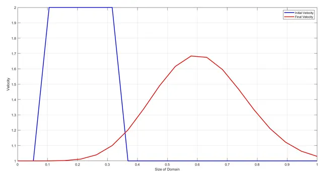
No. of grid points: 20

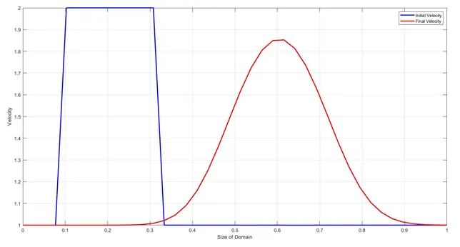
No. of grid points: 40

No. of grid points: 80

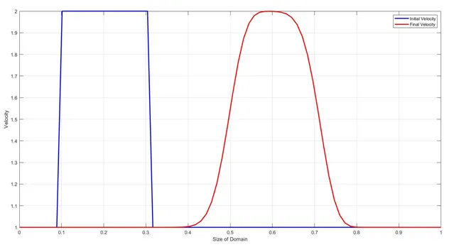
No. of grid points: 160

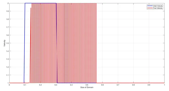
• The results start to blow up as we increase the grid point.
• As the solution progresses from grid point 20 to grid point 160 the artificial diffusion tends to reduce and at the 160 grid point, the solution blows up.

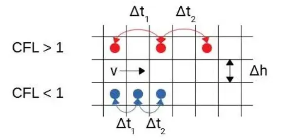
Courant-Friedrichs-Lewy (CFL) condition:

• It is a necessary condition for PDE to solve numerically. It arises in the numerical analysis of the explicit time integration scheme.
• This CFL number determines the level of instability in the particular problem.
• It is basically the stability criterion for a stable solution.
• Any linear explicit convection problem must be equal to or smaller than 1 to give the stable and appropriate solution.

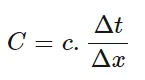
The CFL number is a dimensionless quantity expressed as,

Change in Grid size and stability:

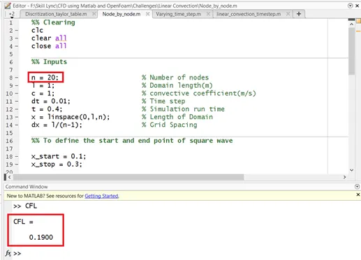
• For grid point 20:
  • The CFL value obtained is 0.19 which is less than 1.

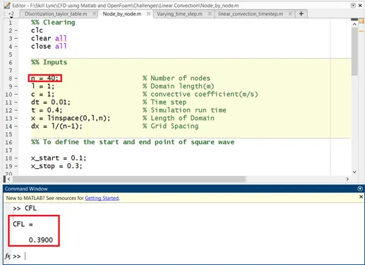
• For grid point 40:
  • The CFL value obtained is 0.39 which is less than 1.

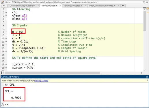
• For grid point 80:
  • The CFL value obtained is 0.79 which is less than 1

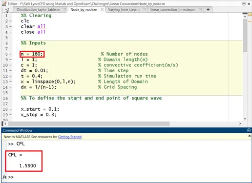
• For grid point 160:
  • The CFL value obtained is 1.59 which is greater than 1.
  • Hence, instability is observed.

CONCLUSION:

• A numerical solution to the one-dimensional linear convection equation is derived and the simulation for a number of nodes 20, 40, 80, and 160 are performed.
• The phenomenon observed in the artificial numerical diffusion, instability, and how the courant and the accuracy of the solution related are clearly explained.
• Change in the grid affects the nature and the stability of the solution is explained.