To plot the P-V graph of Otto cycle and also to find the efficiency of the cycle in MATLAB.

AIM:

Write a program in MATLAB to plot the P-V graph of the otto cycle and also to find the efficiency of the cycle.

GOVERNING EQUATIONS AND THEORY:

• Otto Cycle is an air standard thermodynamic cycle, which well defines the working process of modern days gasoline 4-stroke engines.
• The first person to build the 4-stroke engine was Nicolaus Otto, a German engineer hence given his name as “Otto Cycle”.

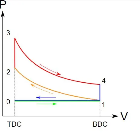
The Pressure-Volume diagram of an Otto Cycle:

• The Otto cycle consists of 4 Standard processes (However 5 processes are involved)
  • Process 0 – 1: Intake Stroke.
  • Process 1 – 2: Isentropic compression.
  • Process 2 – 3: Constant volume heat addition.
  • Process 3 – 4: Isentropic Expansion.
  • Process 4 – 1: Constant volume heat rejection.
  • Process 1 – 0: Exhaust Stroke.

Intake Stroke:

• In the intake stroke, the piston moves from TDC to BDC sucking the air-fuel mixture at constant pressure.

Isentropic Compression and Isentropic Expansion:

• The isentropic process of compression or expansion implies that there will be no inefficiency (loss of mechanical energy), and there be no transfer of heat into or out of the system during that process.

Constant Volume Heat Addition:

• In this process, the heat is added to the system from the external source at constant volume.
• The piston is at TDC at this phase and volume is assumed to be constant (The volume under consideration is clearance volume.

Constant Volume Heat Rejection:

• In this process, the work is done by the system, and heat is ejected to the surrounding.
• The piston is at BDC at thus phase and volume is assumed to be constant (The volume under consideration in total volume i.e., V_clearence+V_swept).

Exhaust Stroke:

• In the intake stroke, the piston moves from BDC to TDC exhaling the burned gases and mixture at constant pressure.

GOVERNING EQUATIONS:

EQUATION OF STATE (IDEAL GAS LAW):

• `PV= γRT`
• `(PV)/T= C` Where: P = Pressur

V = Volume

`γ` = Specific heat ratio = (`C_P/C_v`)

C = Constant

SWEPT VOLUME OF CYLINDER:

• `V_(s )= π/4* D^2*L` Where: `V_s` = Swept volume of cylinder

D = Bore of cylinder

L = Stroke of Piston

CLEARANCE VOLUME OF CYLINDER:

• `V_c= V_s/((C.R-1) )` Where: `V_c` = Clearance Volume

C.R = Compression Ratio

EFFICIENCY OF AN OTTO CYCLE:

• `η= 1-1/((C.R-1) )` Where: `η` = Efficiency

• `V/V_c =1+1/2 (C.R-1)*[R+1-cos⁡θ-(R^2-sin⁡θ^2 )^(1/2) ]`

OBJECTIVE:

1. To study and plot the P-V Diagram of an OTTO Cycle in MATLAB.
2. To find the Thermal Efficiency of the OTTO cycle engine.

In this challenge, we are concern about the plotting of the P-V Diagram of an Otto cycle and to also find the efficiency of the cycle.

INPUTS:

[CODE]

OTTO CYCLE:

% To write the program for otto cycle


clc
clear all
close all


%INPUTS (All are in SI Units)

bore = input('Enter the value of bore dia of Cylinder in meters :');
stroke = input('Enter the value of stroke in meters :');
cr = input('Enter the value of compressionm ratio :');
con_rod = input('Enter the value of length of connecting rod in meters : ');
gamma = input('Enter the value of gamma :');
v_swept = (pi/4)*bore^2*stroke;
v_clearence = v_swept/(cr-1);



% For Isentropic compression (PROCESS 1-2)

p1 = input('Enter the value of P1 for process 1-2 (Isentropic Compression) :');

v1 = v_swept + v_clearence;

t1 = input('Enter the value of T1 for process 1-2 (Isentropic Compression) :');

constant_c = p1*v1^gamma;
V_compression = Piston_kinematics_fun(bore,stroke,cr,con_rod,180,0);

P_compression = constant_c./(V_compression.^gamma);


% For Constant Volume heat Addition (PROCESS 2-3)

v2 = v_clearence;

p2 = p1*(v1/v2)^gamma;

t2 = (p2*v2*t1)/(p1*v1);

v3 = v2;
v0 = v2;

p0 = p1;

t3 = 1000; %- CONSIDERED

p3 = (p2*v2*t3)/(v3*t2);

constant_c = p3*v3^gamma;
V_expansion = Piston_kinematics_fun(bore,stroke,cr,con_rod,0,180);

P_expansion = constant_c./(V_expansion.^gamma);

% For Isentropic Expansion (PROCESS 3-4)

v4 = v1;

p4 = p3*(v3/v4)^gamma;

% For Constant volume heat rejection (PROCESS 4-1)


t4 = (p4*v4*t3)/(p3*v3);

% For finding the efficiency of the otto cycle

term4 = 1/(cr^(gamma-1));

Efficiency = (1-term4)*100

hold on
plot(v0,p0,'*','color','r');
plot(v1,p1,'*','color','g');
plot(v2,p2,'*','color','b');
plot(v3,p3,'*','color','y');
plot(v4,p4,'*','color','k');

hold on
plot([v0 v1],[p0 p1],'g','Linewidth',2);
plot(V_compression,P_compression,'y','Linewidth',2);
plot([v2 v3],[p2 p3],'b','Linewidth',2);
plot(V_expansion,P_expansion,'k','Linewidth',2);
plot([v4 v1],[p4 p1],'r','Linewidth',2);

xlabel('VOLUME');
ylabel('PRESSURE');
title('P-V Diagram');
legend('STATE 0','STATE 1','STATE 2','STATE 3','STATE 4','INTAKE STROKE','ISENTROPIC COMPRESSION','CONSTANT VOLUME HEAT ADDITION','ISENTROPIC EXPANSION','CONSTANT VOLUME HEAT REJECTION');
grid on

OTTO CYCLE FUNCTION:

% This Function Defines the Piston Kinematics.
% Here it gives the values of volume for isentropic compression and
% expansion state.
% Here in this function, change in volume is determined with respect to crank angle. 



function [V] = Piston_kinematics_fun(bore,stroke,cr,con_rod,theta_start,theta_end)
    

        v_swept = (pi/4)*bore^2*stroke;
        v_clearence = v_swept./(cr-1);

        a = stroke/2;
        r = con_rod/a;

        theta = linspace(theta_start,theta_end,100);

        term1 = (cr-1)*0.5;
        term2 = r + 1 - cosd(theta);
        term3 = ((r^2-sind(theta).^2)).^0.5;

        V = (1 + term1.*(term2-term3)).*v_clearence;

    
end

EXPLANATION:

The software used for the programming purpose is MATLAB R2019b.

• The program starts with clc, clear all, close all
  • clc helps in clearing the command window.
  • Clear all, clear all the data in the workspace
  • Close all, close all the window of figure opened in the background.

• Initially, the Otto cycle starts with the from State 0.

STATE 1:

• For making the problem more parametric bore, stroke, compression ratio, length of connecting rod, the value of specific heat ratio, the initial temperature of air-fuel ratio, and initial pressure is taken as input from the user.
• With the help of the user given values value of V_swept and value of V_clearence is calculated.

• v_swept = (pi/4)*bore^2*stroke;

• v_clearence = v_swept/(cr-1);

• Now for calculating the value of ‘V1’

(It is the summation of Swept volume and Clearance volume)

• v1 = v_swept + v_clearence;

• This will give the state 1 values i.e., (P1, V1, T1)

STATE 2:

• From process 1-2 is an ISENTROPIC COMPRESSION

v2 = v_clearence

• For Finding P2:

Therefore,

• p2 = p1*(v1/v2)^gamma; (This will give the value of P2)

• Hence by the Ideal gas law,

`(PV)/T= C`

• Therefore,
• t2 = (p2*v2*t1)/(p1*v1); (This will give value of T2)

• This will give the state 2 values i.e., (P2, V2, T2)

STATE 3 and STATE 4:

• Similarly, state 3 (Isentropic compression) and state 4 (Constant volume heat addition) will be calculated.
• Details are shown in the code.
• Now, for calculating the exact P-V graph of the otto cycle, a separate function is defined, which will calculate the process flow points and will generate the Isentropic compression and Isentropic Expansion graph at 0 to 180 and 180 to 0 degree of crank angle respectively.

For Isentropic Compression: (Crank Angle 0 - 180 Deg).

constant_c = p1*v1^gamma;

V_compression = Piston_kinematics_fun(bore,stroke,cr,con_rod,180,0);

P_compression = constant_c./(V_compression.^gamma);

For Isentropic Expansion: (Crank Angle 180 - 0 Deg).

constant_c = p3*v3^gamma;

V_expansion = Piston_kinematics_fun(bore,stroke,cr,con_rod,0,180);

P_expansion = constant_c./(V_expansion.^gamma);

OTTO CYCLE FUNCTION:

`V/V_c =1+1/2 (C.R-1)*[R+1-cos⁡θ-(R^2-sin⁡θ^2 )^(1/2) ]`

• This Equation is used to calculate the volume of compression and expansion stroke.
• Hence in the otto cycle function, this will define the value of volume at various instances during compression and expansion stroke concerning crank angle.

term1 = (cr-1)*0.5;

term2 = r + 1 - cosd(theta);

term3 = ((r^2-sind(theta).^2)).^0.5;

V = (1 + term1.*(term2-term3)).*v_clearence;

For finding the efficiency of the Otto cycle:

• The efficiency of the cycle is the function of the compression ratio.
• The efficiency of the cycle is found out by using the following formula

`η= 1-1/((C.R-1) )`

Therefore, term4 = 1/(cr^(gamma-1));

Efficiency = (1-term4)*100

Plot command is used to plot all the various states and to display the process flow from various point locations.

plot(v0,p0,'*','color','r');

plot(v1,p1,'*','color','g');

plot(v2,p2,'*','color','b');

plot(v3,p3,'*','color','y');

plot(v4,p4,'*','color','k');

This will plot the points of various states.

plot([v0 v1],[p0 p1],'g','Linewidth',2);

plot(V_compression,P_compression,'y','Linewidth',2);

plot([v2 v3],[p2 p3],'b','Linewidth',2);

plot(V_expansion,P_expansion,'k','Linewidth',2);

plot([v4 v1],[p4 p1],'r','Linewidth',2);

This will plot the curves of various states.

COMMAND WINDOW INPUTS:

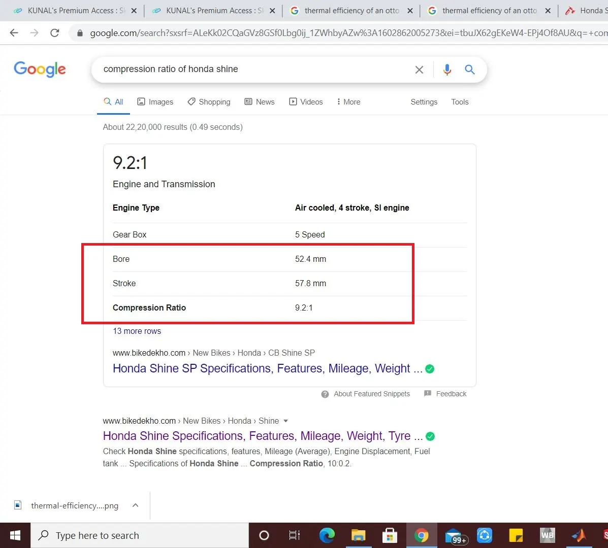
The input data was considered for Honda Shine 125cc 4-Stroke Engine (Source - Internet)

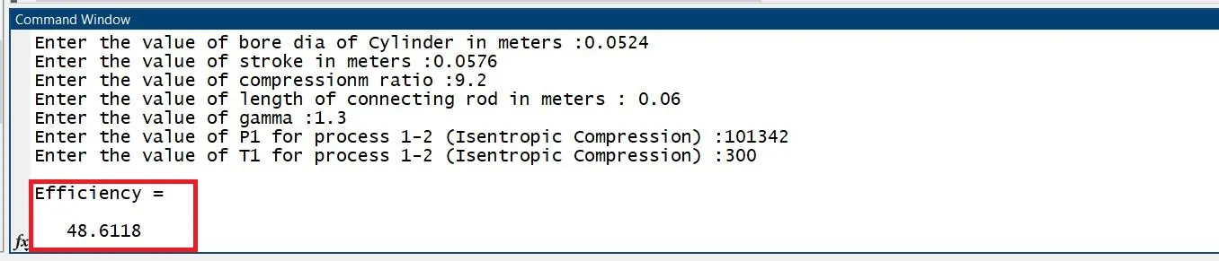
The efficiency of the Otto Cycle at particular inputs is 48.61 %

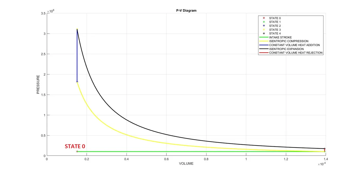
P-V Diagram of Otto Cycle at Respective inputs.

CONCLUSION:

• Hence using MATLAB, we are able to calculate the P-V Diagram for an Otto Cycle.
• The efficiency of the Otto cycle is also calculated.