WEEK – 3 SOLVING SECOND ORDER ODEs

AIM:

Write a program in MATLAB to solve the Second Order ODEs

GOVERNING EQUATIONS AND THEORY:

• In Engineering, ODE is used to describe the transient behavior of a system.
• There are 100s of ODESs which are used to solve real-life engineering problems in an exact and accurate way.
• One of the examples of such ODEs is of a simple pendulum.
• The way the pendulum moves depends on Newton's second law. When this law is written down, we get a second order Ordinary Differential Equation that describes the position of the "ball" w.r.t time.

This ODE represents the equation of motion of a simple pendulum with damping.

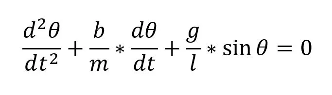
Here, b = Damping coefficient.

g = Acceleration due to gravity (9.81 m/s²).

L = Length of the Pendulum.

m = Mass of the sphere attached at one end.

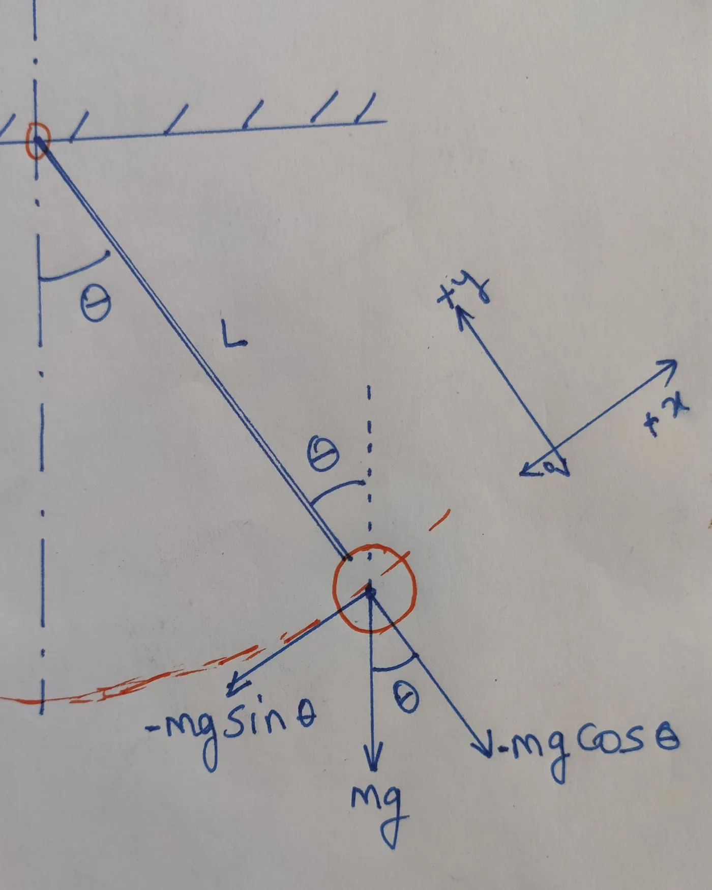
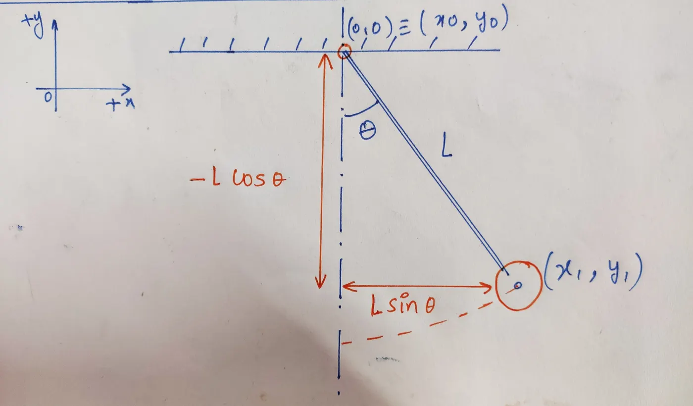
• Now for defining this into MATLAB, the above ODE has to be differentiated.
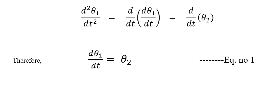
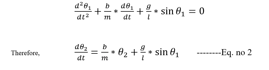
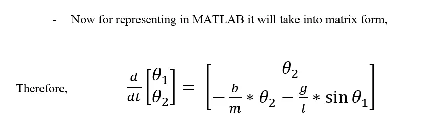
  • As the above ODE is of second order, hence it has to break down into two separate first-order ODEs.
  • Now here the simple pendulum is the function of Angular_Displacement and Angular_Velocity.
• Angular_Displacement = `θ_1`
• Angular_Velocity =`θ_2`

• Hence, for converting it into first-order derivatives,

OBJECTIVE:

1. To solve the Second Order ODE for a pendulum in MATLAB.
2. To plot the amplitude time graph and study the behavior.
3. To plot the animation of the simple pendulum using the same generated output.

INPUTS:

[CODE]

SECOND ORDER ODE (PENDULUM):

clc
clear all
close all


b = 1;
g = 9.81;
l = 1;
m = 1;

theta = [0;3];

t_span = linspace(0,20,200);

[t,results] = ode45(@(t,theta) ode_func(b,g,l,m,theta),t_span,theta);

figure(1);
plot(t,results);
xlabel('------TIME------');
ylabel('--------AMPLITUDE---------');
legend('ANGULAR DISPLACEMENT','ANGULAR VELOCITY');
grid on

videofile = VideoWriter('Second Order ODE of Pendulum.avi');
open(videofile);

for i = 1:length(t_span)
    angular_displacement = results(i,1);
    
    x0 = 0;
    y0 = 0;
    
    x1 =  l*sin(angular_displacement);
    y1 = -l*cos(angular_displacement);
    
    figure(2)
    plot(x0,y0,'o','Markersize',12);
    hold on
    plot([x0 x1],[y0 y1],'b','Linewidth',3);     
    plot(x1,y1,'o','Markersize',25,'MarkerFaceColor','y');
    hold off  
    
    axis([-1.5 1.5 -1.5 1.5]);
    
    M = getframe(gcf);
    writeVideo(videofile,M);
        
end

close(videofile);

ODE FUNCTION:

% Here, this function determines the angular displacement and angular
% velocity of the pendulum


function [dtheta_dt] = ode_func(b,g,l,m,theta)

    theta_1 = theta(1);
    theta_2 = theta(2);
    
    dtheta1_dt = theta_2;                                 % This will define the Angular displacement.
    dtheta2_dt = -(b/m)*theta_2 - (g/l)*sin(theta_1);     % This will define the angular velocity.
    
    dtheta_dt = [dtheta1_dt;dtheta2_dt];
    

end

EXPLANATION:

The software used for the programming purpose is MATLAB R2019b.

• The program starts with clc, clear all, close all
  • clc helps in clearing the command window.
  • Clear all, clear all the data in the workspace
  • Close all, close all the window of figure opened in the background.

• Initially the values of b, g, l and m are defined.
• As mentioned in the problem statement, angular_displacement starts from 0, angular_velocity starts from 3 and time_span is from 0 to 20 sec with 200 intervals.

• Hence,
  • theta = [0;3];
  • t_span = linspace(0,20,200);

• Solver “ode45”:
  • Solver ode45 is an inbuilt function in MATLAB use to solve the differential equations.
  • This is used in our code to solve the second order ODE.

[t,results] = ode45(@(t,theta) ode_func(b,g,l,m,theta),t_span,theta);

• Above, ode_function is been defined in another code, where it generated the value of angular displacement and angular velocity respectively by solving the first order ODE and stores the value in results.
• For making the problem more parametric bore, stroke, compression ratio, length of connecting rod, value of specific heat ratio, initial temperature of air-fuel ratio, and initial pressure is taken as input from the user.
• For generating the amplitude vs time graph, plot command is used.

figure(1);

plot(t,results);

xlabel('------TIME------');

ylabel('--------AMPLITUDE---------');

legend('ANGULAR DISPLACEMENT','ANGULAR VELOCITY');

grid on

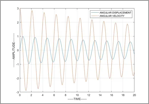
• For the given value of damping coefficient in challenge (b = 0.05), following graph is obtained.

Further, as we change the values of damping coefficient, following graphs were obtained:

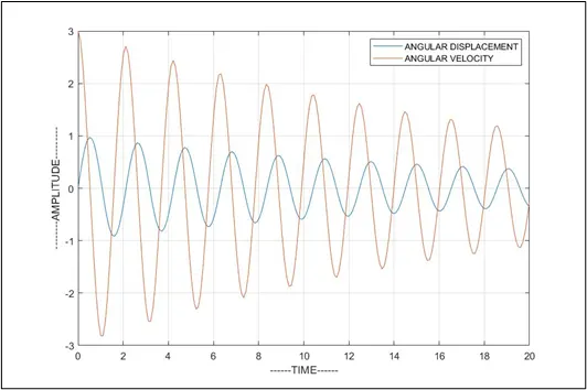
• For the value of coefficient of damping (b = 0.1) following graph is obtained.

• For the value of coefficient of damping (b = 0.5) following graph is obtained.

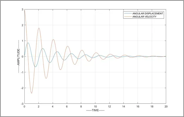
• For the given value of coefficient of damping (b = 0.8) following graph is obtained.

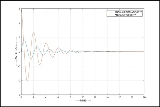
• Now for plotting the pendulum, for loop is implemented.
• The values of e., Angular displacement from generated results is feed into the variable, angular_displacement.
  • angular_displacement = results(i,1)
• This will give the values of angular displacement in array form.

Anatomy of simple Pendulum:

• In simple pendulum, a bob of mass ‘m’ is suspended from a string of length ‘L’, from one pin point ‘O’.
• Hence for creating such anatomy following command were executed in MATLAB.
• Here X0, Y0 defines the position of the pin from where the string is suspended.
• X1, Y1 are the end points where the bob of mass ‘m’ is attached.
• ‘Markersize’, This command is used to plot the pin point of pendulum and to plot the bob.
• For creating the animation VideoWrite command is used.

Output Video File:

You can find the link of the video of pendulum below (For b = 0.05)

https://youtu.be/EyJ91kFZQL8

CONCLUSSION:

1. Hence, calculations of Second Order ODE for pendulum is been performed using MATLAB.
2. Plotting of amplitude and time graph is been done, and animation of pendulum is been plotted.