2R ROBOTIC ARM CHALLENGE IN MATLAB

AIM: Write a program in MATLAB to simulate the forward kinematics of a 2R Robotic Arm.

GOVERNING EQUATIONS AND THEORY:

• Kinematics is the branch of science in which we study the possible motion of a body or the group of bodies without considering external force applied.

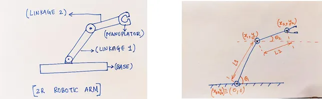
• Kinematics has a wide application in robotic Engineering.

• Mainly there are two types:

1. Forward Kinematics
2. Inverse Kinematics

FORWARD KINEMATICS:

• Forward kinematics is mainly used to calculate the position of the end effectors when we know the angles of each joint.

INVERSE KINEMATICS:

• Inverse Kinematics is mainly used to calculate the angle of each joint when the position of the end effector is known.

ROBOTIC ARM:

• The robotic arm is mainly the programmable machine that is invented for the reduction of human effort and to increase in ease of operation.
• The robotic Arm is a highly parametric machine that can be coded and programmed according to application and use.

OBJECTIVE:

1. To study the forward kinematics of the robotic arm.
2. To create an animation file of the plot.
3. To determine the workspace of the robotic arm.

In this challenge we are concern about the 2R Robotic arm, this 2R robotic arm has two kinematic linkages and rotational movements.

INPUTS:

[CODE]

% WRITE A PROGRAM IN MATLAB TO SIMULATE THE FORWARD KINEMATICS OF THE 2R ROBOTIC ARM.
% ALSO TO PLOT THE DATA AND TO CREATE AN ANIMATION FILE OF THE PLOT.
 
clc
close all
clear all
 
 
 
l1 = 2;
l2 = 1;
 
theta1 = linspace(0,90,10);
theta2 = linspace(0,80,60);
 
videofile = VideoWriter('robotic_arm.avi');
open(videofile);
 
for i = 1:length(theta1)
    
    for j = 1:length(theta2)
        
        x0 = 0;
        y0 = 0;
        
        x1 = l1*cosd(theta1(i));
        y1 = l1*sind(theta1(i));
 
        x2 = x1 + l2*cosd(theta2(j));
        y2 = y1 + l2*sind(theta2(j));
       
        plot([x0 x1],[y0 y1],[x1 x2],[y1 y2],'Linewidth',3);
        
        axis([0 3 0 3]);
        title('FORWARD KINEMATICS OF 2R ROBOTIC ARM');
        xlabel('X AXIS');
        ylabel('Y AXIS');
        grid on
 
        pause(0.01);

        M = getframe(gcf);
        writeVideo(videofile,M);
        
    end
end
 
close(videofile);

EXPLANATION:

The software used for the programming purpose is MATLAB R2019b.

• The program starts with clc, clear all, close all
  • clc helps in clearing the command window.
  • Clear all, remove all the data in the workspace
  • Close all, close all the window of figure opened in the background.

• Initially, we have to give the values of the length of the linkages.
  • L1 defines the length of linkage 1.
  • L2 defines the length of linkage 2.

• theta1 and theta2 are the angles of the linkage with respect to horizontal.
  • theta1 is the angle of link 1 with the horizontal.
  • theta2 is the angle of link 2 with the horizontal.
  • Therefore, for taking the multiple values of both the theta, the linspace command is used.

• Hence, theta1 = linspace (0,90,10)

theta2 = linspace (0,80,60)

• Here, 0 is the starting angle, 90 and 80 are the ending angle of theta1 and theta2 respectively and 10 & 60 are the number of divisions in which theta1 and theta2 are bifurcated.
• Now, here it is difficult to write a program for 10 * 60 = 600 values, so here for loop command is used to super ease the operation.

• Hence, for i = 1:length(theta1), this defines the value to theta1 for variable inputs.

• Similarly, for each value of theta1, there will be 60 values of theta2, hence for this another for loop will be required.

• Hence for i = 1:length(theta2), this defines the value of theta2 for variable inputs

• Origin of link1 is defined, x0 = 0, y0 = 0

• x1, y1, and x2, y2 are the coordinates of the endpoint of the link1 and link2.

• x1, y1 are define in the for loop as follows:

• x1 = l1*cosd(theta1(i)); [Here, cosd(theta1) is defined, as MATALB takes the value in radian]

• y1 = l1*sind(theta1(i)); [Here, sind(theta1) is defined, as MATALB takes the value in radian]

• Similarly, x2, y2 are also defined:

• x2 = x1 + l2*cosd(theta2(i));

• y2 = y1 + l2*sind(theta2(i));

• plot command is used for plotting the graph.

• plot([x0 x1],[y0 y1],[x1 x2],[y1 y2],'Linewidth',3);

• To display the axis, the axis command is defined according to the length of the two links.
  • axis([0 3 0 3])
• xlabel, ylabel commands are used to display the labels in the axis.

• pause(0.01), this pause command is used to plot the different graphs into one single animation.

• Now to create an animation (.AVI) file, the following errors were encountered.
  • ERROR 1:

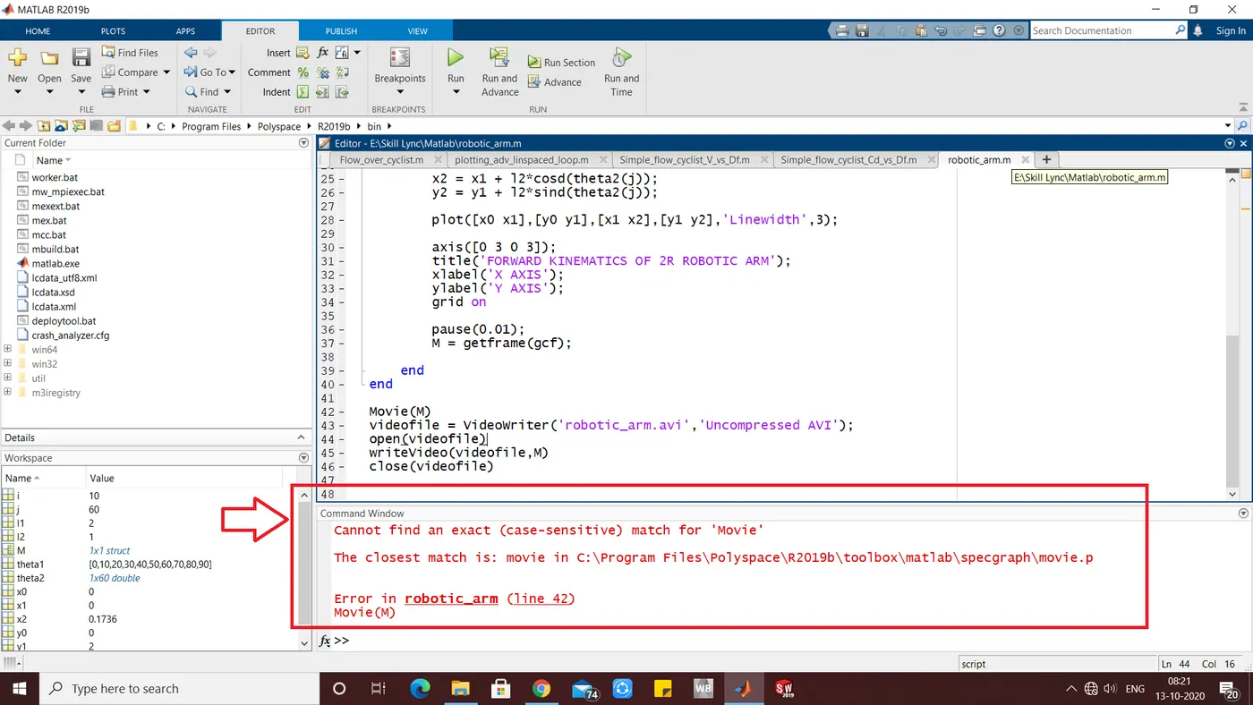
• As the MATLAB is a case sensitive language, hence while creating the movie it showed this error, so I fixed it.
• But while figuring out the program, I got to know that there was no use of movie(M) expression, so I removed it.
  • ERROR 2:

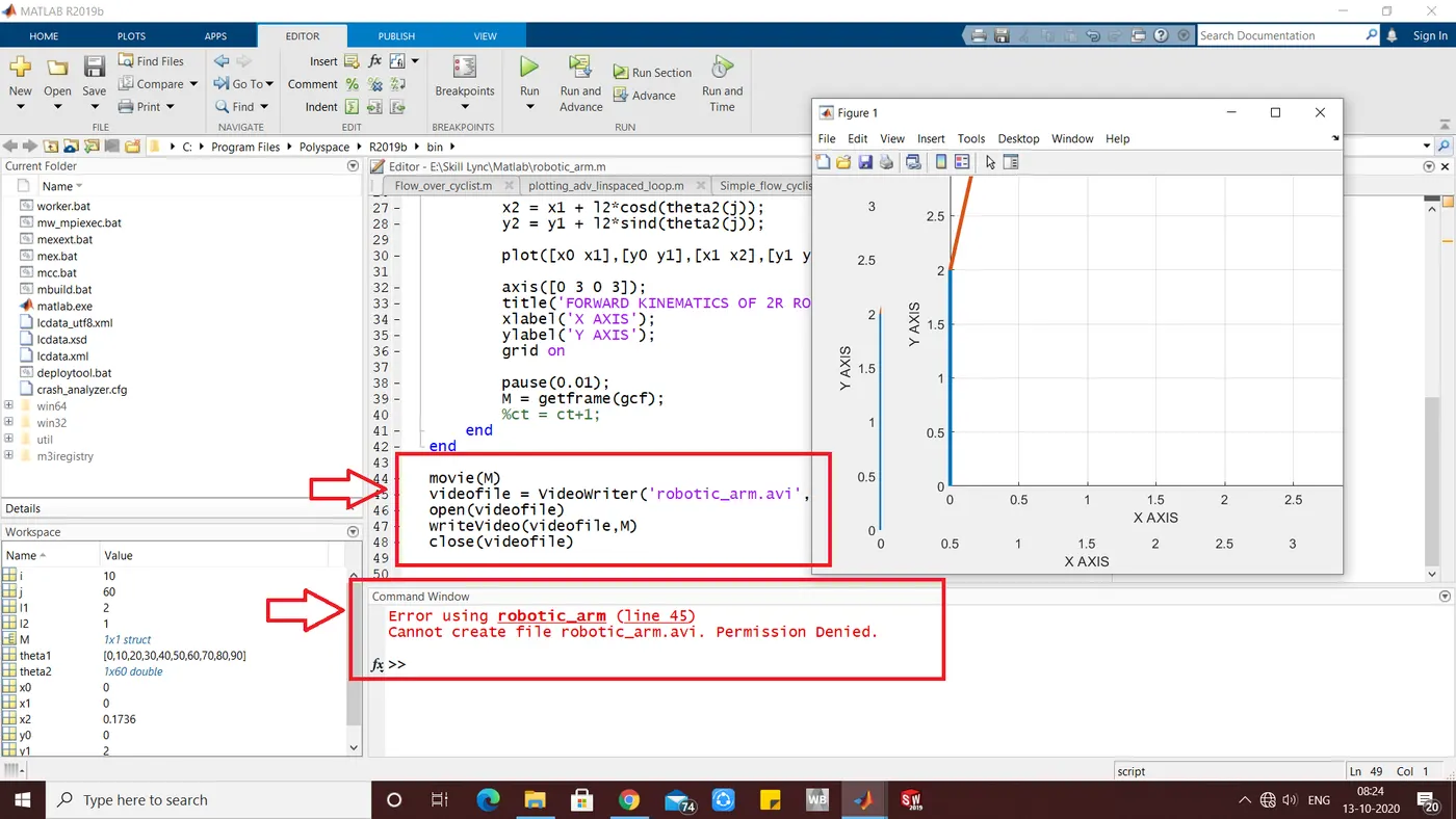
• It showed permission denied to create the animation of the program, so after a couple of trials, I searched in the command window help VideoWriter and I found something interesting, following is the image of the updated commands.

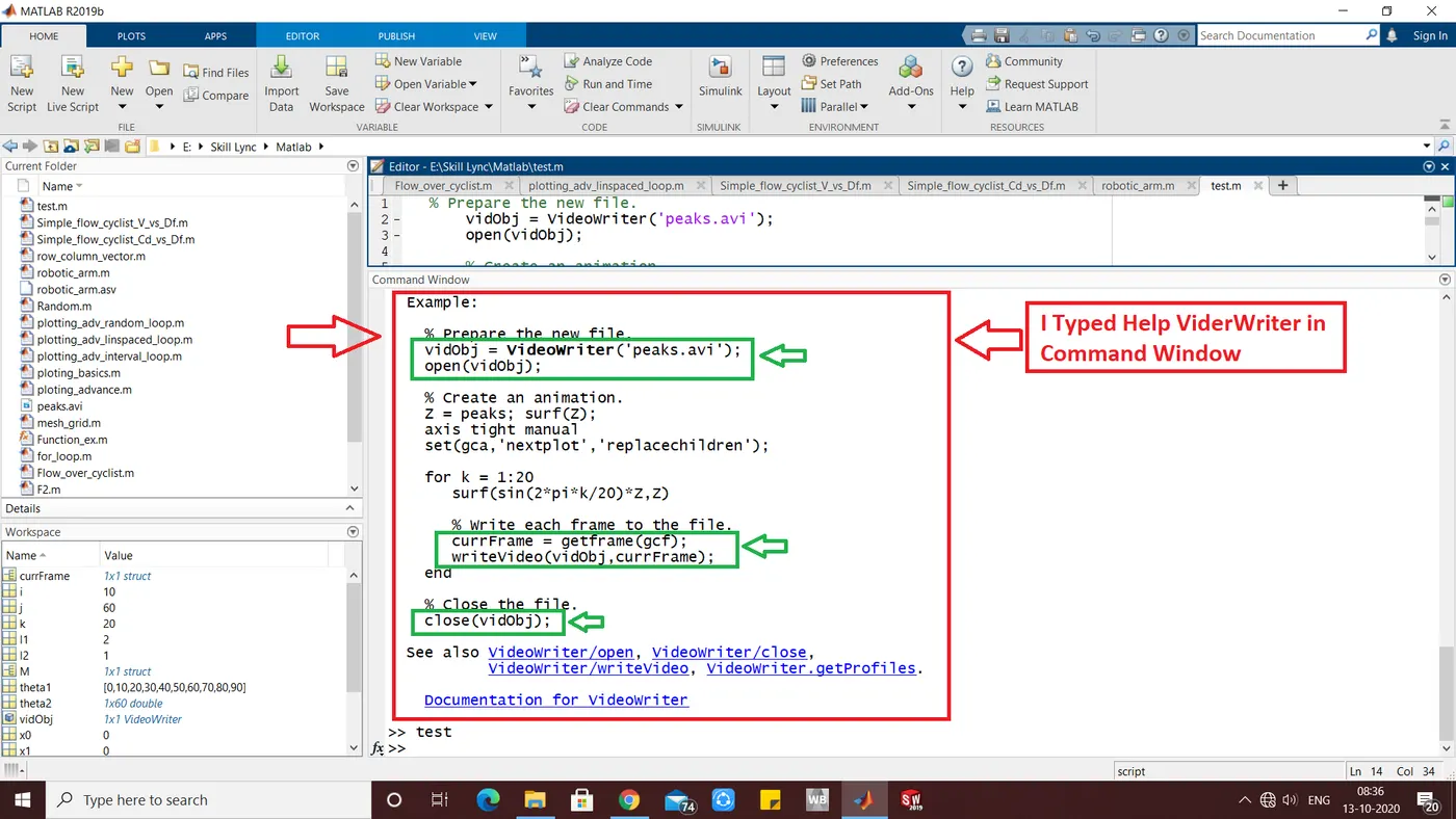
• Hence, I was using the correct command, but now I interchanged the positions of the commands.
• I put the writeVideo(videofile,M) file into the loop, where it will be creating the movie frame by frame and will convert it into animation.
• At the end of the task, it will close the videoWriter.
• The correct command rearrangement is shown in the code.

Animation of the robotic arm is been uploaded on YouTube, please find the link below.

https://youtu.be/8QECM79Nguk

CONCLUSION:

• For different angles of link1, various combinations of Link2 is possible.
• We can identify the various possible workspace of a robotic arm.