Week 4.1 - Genetic Algorithm
Genetic Algorithm:
stalagmite function Program:
function [f] = stagalmite (input_vector)
x= input_vector(1);
y=imput_vector(2);
f1=(sin(5.1*pi*x+0.5)).^6;
f2=exp((-4*log(2)*((x-0.0667).^2))/0.64));
f3=(sin(5.1*pi*y+0.5)).^6;
f4=exp((-4*log(2)*((y-0.0667).^2))/0.64));
A = -(f1*f2*f3*f4);
end
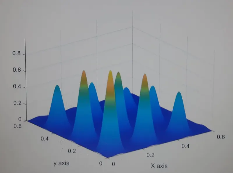
- The negative command is used in the program in order to invert the plot as the ga command finds only the minimum point.
Main program:
close all
clear all
clc
%input
x = linspace(0,0.6,150);
y = linspace(0,0.6,150);
[xx,yy] =meshgrid(x,y);
for i=1:length(xx)
for j=1:length(yy)
input_vector(1)= xx(i,j);
input_vector(2)= yy(i,j);
f(i,j) = stalagmite(input_vector);
end
end
surfc(xx,yy,f)
shading interp
[inputs, fval ] = ga(@stalagmite,2)
Xlabel (‘x axis’)
Ylabel (‘y axis’)
Study-1 statistical behaviour:
num_spaces=50
tic
for i=1:num_spaces
[results,fopt(i)] = ga(@stagalmite,2)
xopt(i)=results(1)
yopt(i)=results(2)
end
study_time1=toc;
mean=-(mean(fopt))
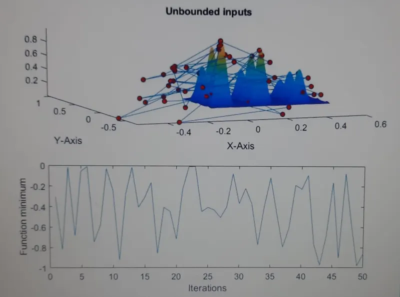
figure(1)
subplot(2,1,1)
hold on
surf(x,y,-f)
shading interp
plot3(xopt,yopt,-fopt,'marker','0')
title(‘unbounded inputs’)
subplot(2,1,2)
plot(fopt)
xlabel('iterations')
ylabel('function minimum')
Study-2 Statistical behaviour with upper and lower limits:
tic
for i=1:num_spaces
[results,fopt(i)] = ga(@stagalmite,2,[],[],[],[],[0;0],[1;1]);
xopt(i) = results(1);
yopt(i) = results(2);
end
study_time2=toc
mean=-(mean(fopt))
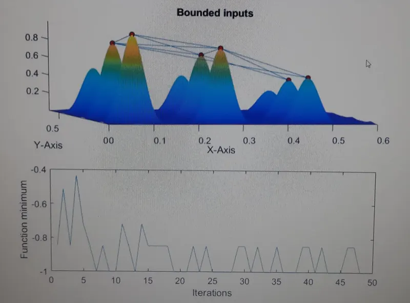
figure(2)
subplot(2,1,1)
hold on
surf(x,y,-f)
shading interp
plot3(xopt,yopt,-fopt,'marker','o')
title(‘Bounded inputs’)
subplot(2,1,2)
plot(-fopt)
xlabel('iterations')
ylabel('Function minimum')
Study-3 Increasing GA Iterations:
options= optimoptions ('ga')
options= optimoptions(options,'populationsize',400);
tic
for i = 1:num_spaces
[results,fopt(i)] = ga(@stagalmite, 2, [],[],[],[],[0;0],[1;1],[],[],options)
xopt(i) = results(1)
yopt(i) = results(2)
end
study_time3=toc;
mean=-(mean(fopt))
figure(3)
subplot(2,1,1)
hold on
surf(x,y,-f)
shading interp
plot3(xopt,yopt,-fopt,'marker','o')
subplot(2,1,2)
plot(fopt)
xlabel('iterations')
ylabel('function minimum')
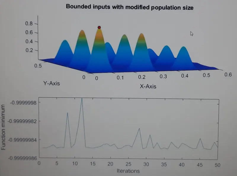
Result:
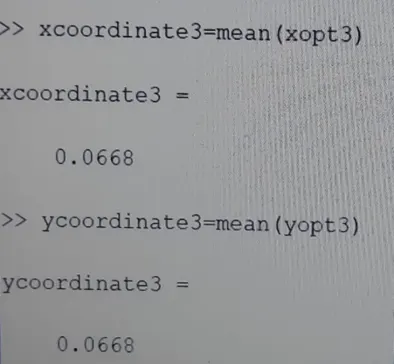
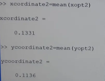
The time taken for the study, global maximum value and the coordinate values of x and y are found out for each study and the results are shown below:
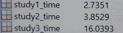
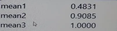
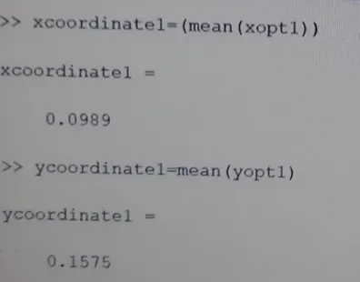
 .
.