Week 4.1 - Genetic Algorithm
AIM:
- Write a code to optimise the stalagmite function and find the global maxima of the function using matlab.
CONCEPT:
- Genetic Algorithms are inspired by Charles Darwin’s theory: “Natural selection is survival of the fittest”. The term fit refers to the success of reproduction or, in other words, the capability of creating offsprings for successive generations.
- The concept of biological evolution is used to solve all different kinds of problems and has become well-known for its reliable global search capabilities. Thus, genetic algorithms have been used to solve myriads of real-world optimization problems and are an essential subject of research in optimization and related fields.
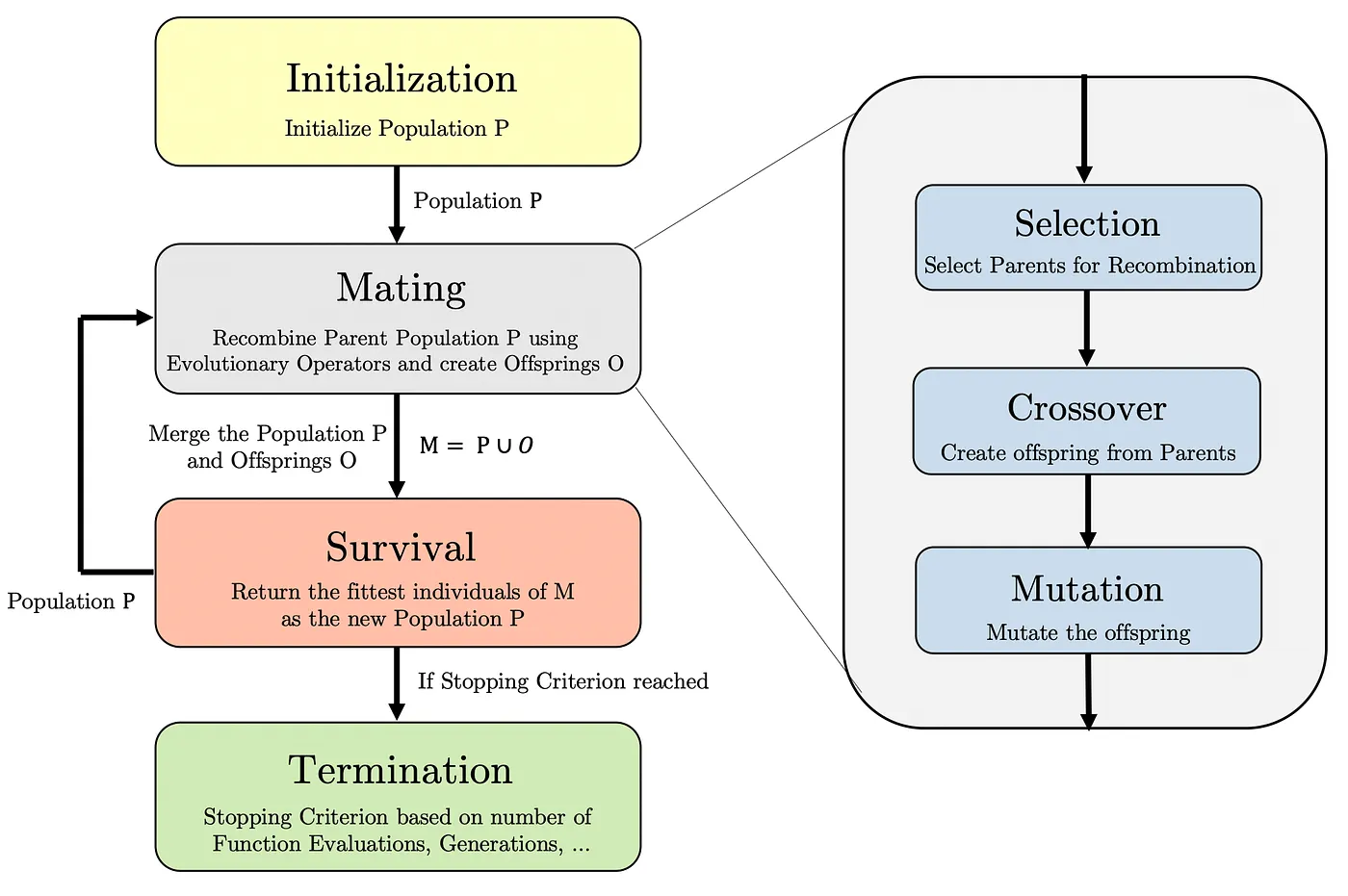
- Evaluate: The actual problem to be solved, where the function determines the fitness of each individual.
- Initialize: This method returns the initial population P.
- Selection: A function returning the individuals in the population functioning as parents for recombination.
- Crossover: A function creating one or multiple offsprings given two or more parents.
- Mutation: A method mutation each offspring with a specific probability.
- Survival: A function reducing the merged population to a set of solutions equal to the population size by applying the principle of survival of the fittest
BODY OF THE CONTENT:
{SOFTWARE USED - MATLAB}
PROGRAM OF 'GENETIC ALGORITHM' USING STALAGMITE FUNCTION
close all
clear all
clc

% Defining our search space
x = linspace(0,0.6,150);
y = linspace(0,0.6,150);

% Evaluating the stalagmite function
for i = 1:length(x)
    for j = 1:length(y)
        input(1) = x(i);
        input(2) = y(j);
        f(i,j) = stalagmite(input);
    end
end

num_case = 50;

tic
% Case Study 1: Simple function without any bounds
for k = 1:num_case
    [input, fopt(k)] = ga(@stalagmite,2);
    xopt(k) = input(1);
    yopt(k) = input(2);
end

figure(1)
subplot(2,1,1);
surfc(x,y,-f);
shading interp
hold on
plot3(xopt,yopt,-fopt,'marker','o','MarkerSize',6,'MarkerFaceColor','r');
subplot(2,1,2);
plot(fopt);
title('Optimization without bounds');
xlabel('Iteration');
ylabel('F Maximum');

study_1 = toc

tic
% Case Study 2: Given the lower and upper bounds
for k = 1:num_case
    [input, fopt(k)] = ga(@stalagmite,2,[],[],[],[],[0;0],[0.4;0.4]);
    xopt(k) = input(1);
    yopt(k) = input(2);
end

figure(2);
subplot(2,1,1);
surfc(x,y,-f);
shading interp
hold on
plot3(xopt,yopt,-fopt,'marker','o','MarkerSize',6,'MarkerFaceColor','r');
subplot(2,1,2);
plot(fopt);
title('Optimization with upper and lower bounds');
xlabel('Iteration');
ylabel('F Maximum');
study_2 = toc

tic
% Case Study 3: Maximizing the population size to optimize the result
options = optimoptions('ga');
options = optimoptions(options,'PopulationSize',270);
for k = 1:num_case
    [input,fopt(k)] = ga(@stalagmite,2,[],[],[],[],[0;0],[0.4;0.4],[],options);
    xopt(k) = input(1);
    yopt(k) = input(2);
end

figure(3)
subplot(2,1,1);
surfc(x,y,-f);
shading interp
hold on
plot3(xopt,yopt,-fopt,'marker','o','MarkerSize',6,'MarkerFaceColor','r');
subplot(2,1,2);
plot(fopt);
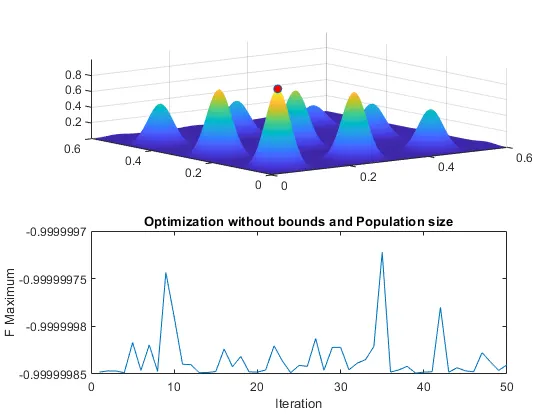
title('Optimization without bounds and Population size');
xlabel('Iteration');
ylabel('F Maximum');
study_3 = toc
FUNCTION CODE OF STALAGMITE
function f = stalagmite(input)

x = input(1);
y = input(2);

f1x = (sin((5.1*pi*input(1)) + 0.5))^6;
f1y = (sin((5.1*pi*input(2)) + 0.5))^6;

f2x = exp((-4*log(2))*((input(1) - 0.0667)^2/0.64));
f2y = exp((-4*log(2))*((input(2) - 0.0667)^2/0.64));

f = -(f1x*f2x*f1y*f2y);

end
EXPLANATION OF CODE:
- In this code i am trying to find the 'Global maxima of ga'.
- close all, clear all, clc are the basic commands of the program.
- close all - Close all figures whose handles are visible.
- clear all - To clear all the variables from the current workspace.
- clc - Clear all the texts from the command window.
- Defining the search space of x and y with the help of linspace command which we are going to perform 'ga'.
- linspace - The linspace function generates linearly spaced vectors.
- Next with a help of the for loop and stalagmite function I created the the massive matrix of 'f'.
- num_case - defining the number of cases that we are going to perform the optimization is set to '50 times'.
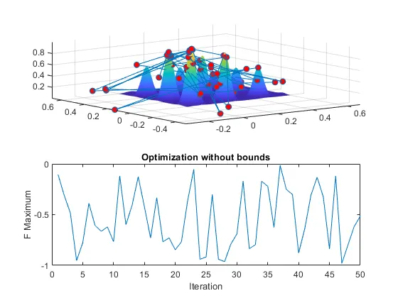
- In the study 1 unconstrained 'ga function' without any bound discussed x = ga(fun,nvars)
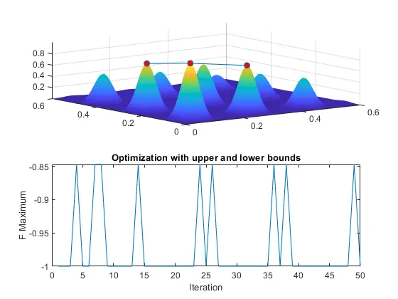
- In the study 2 'ga function' with lower and upper bound discussed,x = ga(fun,nvars,A,b,Aeq,beq,lb,ub).
- In the study 3 'ga function' with condition of population target, x = ga(fun,nvars,A,b,Aeq,beq,lb,ub,nonlcon,options)
- In the final study that helps to get the result of 'GLOBAL MAXIMA' Value.
- tic&toc - This command used to calculate the time of each and every study.
- using for loop for the case 1 and get the optimum values of x,y,f, this helps to show the point markers in the graph
- subplot - This is the inbuilt option to split the figure window into multiple pieces
- shading interp - which is used to hide the grid lines in the '3D'plot figure.
- title - For giving title to the graph.
- plot3 - This command is used to Plot Graphs in '3D'
- xlabel & ylabel - Used to name the 'xaxis' and 'yaxis' in the diagram.
Common GA syntax - Find global minima & maxima
1. Unbound constrains
2. With lower and upper bounds
3. Population included
ERRORS WHILE PROGRAMING:
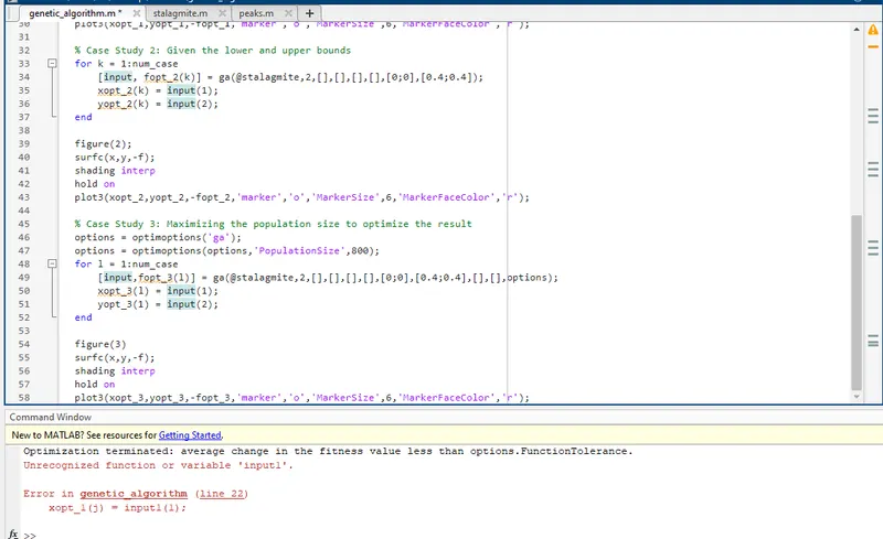
- I missed the variable indexing of input command, i faced this error and i correct it, after that the error resolved
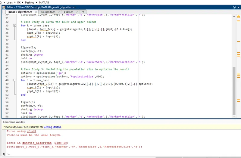
- In this error i missed to give the length of fopt, after that i correct it the problem resolved.
CONCLUSION:
- On the conclusion of this program it helps me to learn how to use the 'global optimisation' function in matlab
- global optimisation is one of the best method for optimisation, it has wide range of properties.