Week 4.1 - Genetic Algorithm

AIM : To study about Genetic Algorithm and to calculate the global maxima of stalagmite function using Genetic Algorithm in MATLAB.

OBJECTIVE :

• To study about Genetic Algorithm and Stalagmite function.
• To write a code in Matlab to optimise the stalagmite function and find the global maxima of the function.
• To plot graphs based on the studies done for Genetic Algorithm.

THEORY :

Concept of Genetic Algorithm –

The Genetic Algorithm works on the process of natural selection where the fittest individuals are selected for reproduction in order to produce offspring of the next generation. It is a method for solving both constrained and unconstrained optimization problems that is based on natural selection. The algorithm begins by creating a random initial population of individual selections and it keeps on modifying this population repeatedly creating a sequence of new population.

Stalagmite Function

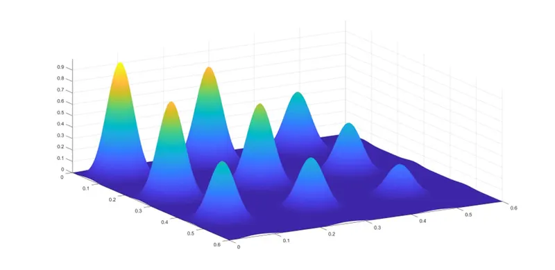
Stalagmite function is a mathematical model which helps to generate local minima and maxima. It is a three-dimensional function and the way the function is designed is that it has a lot of local maxima or minima and one global maxima or minima. The name stalagmite is actually a type of rock formation that arises from the floor of a cave due to the accumulation of material deposited on the floor from ceiling drippings.

The stalagmite function is given in matlab as,

f1,x=[sin(5.1πx+0.5)]6f1,x=[sin⁡(5.1πx+0.5)]6

f1,y=[sin(5.1πy+0.5)]6f1,y=[sin⁡(5.1πy+0.5)]6

f2,x=exp[−4ln(2)(x−0.0667)20.64]f2,x=exp⁡[-4ln⁡(2)(x-0.0667)20.64]

f2,y=exp[−4ln(2)(y−0.0667)20.64]f2,y=exp⁡[-4ln⁡(2)(y-0.0667)20.64]

∴∴f(x,y)=f1,x×f1,y×f2,x×f2,yf(x,y)=f1,x×f1,y×f2,x×f2,y

Explanation of code:

The code starts with clear all, close all and clc where ''clear all'' command is used to clear the data stored in the workspace, ''close all''command is used to close all plots and figures,''clc'' command is used to clear the command window.Then the ‘x’ array and ‘y’ array is defined using ‘linspace’ command to create values at 150 equal intervals.A 2D mesh of x and y array is created by using ‘meshgrid’ command and the number of iterations or cases that the code should perform is defined. This is given by n = 50.To evaluate the stalagmite function, ‘for’ loop is used where ‘i’ is initialized and for every value of ‘i’ another ‘for’ loop is used to initialize ‘j’ we are used two for loops .The input vector values of ‘xx’ and ‘yy’ are defined and the stalagmite function for these input vectors is defined. This will form a basic .Then the function created in the loop is plotted by using ‘surfc’ command for ‘xx, yy and function output’. To neglect the gridlines on the surface and obtain a smooth and clean plot, ‘shading interp’ command is used. The ‘subplot(2,1,1)’ is used to plot multiple plots on same figure which also divides figure in grid of 2x1 and axes to be placed at 1.The results of the above case will be different for each time we run the program. To get same value each time, we need to restrict the program within specific bounds namely upper bound and lower bound. The procedure for coding and plottind this procedure is same as Study 1. The only difference is in the ‘ga’ syntax. This time the algorithm is provided lower limits and upper limits as [0;0] and [1;1] respectively.After plotting the results for Study 2 or the bounded case, it is observed that the results are not same every time the program terminates. A solution to this problem is to increase the number of cases or iterations.The syntax for ‘ga’ contains ‘option’ term and the rest of the code is same as for Study 1 and 2.

%Define Stalagmite Function

function [f] = stalagmite(input_vector)
x = input_vector(1);
y = input_vector(2);

t1 = (sin((5.1*pi*x)+0.5))^6;
t2 = (sin((5.1*pi*y)+0.5))^6;
t3 = exp(-4*log(2)*((x-0.0667)^2)/0.64);
t4 = exp(-4*log(2)*((y-0.0667)^2)/0.64);

f = -(t1*t2*t3*t4);
end

clear all
close all
clc

%Definie our search space
x = linspace(0,0.6,150);         %x array
y = linspace(0,0.6,150);         %y array
n = 50;                          %number of cases

%Creating a 2D mesh
[xx yy] = meshgrid(x,y);

%Evaluating a stalagmite function
for i = 1:length(xx)
    for j = 1:length(yy)
        input_vector(1)=xx(i,j);
        input_vector(2)=yy(i,j);
        f(i,j) = stalagmite(input_vector);
    end
end

%Study 1 : Statistical Behaviour

tic
for i = 1:n
    [inputs,fopt(i)] = ga(@stalagmite,2);
    xopt(i) = inputs(1);
    yopt(i) = inputs(2);
end
study1_time = toc

figure(1)
subplot(2,1,1)
hold on
surfc(xx,yy,-f)
shading interp
xlabel('X-axis')
ylabel('Y-axis')
title('Statistical Behaviour with Unbound inputs')
plot3(xopt,yopt,-fopt,'marker','o','markersize',5,'markerfacecolor','r')
subplot(2,1,2)
plot(-fopt)
xlabel('No. of Iterations')
ylabel('Function maximum')

%Study2 : Statistical behaviour with upper and lower bounds

tic
for i = 1:n
    [inputs,fopt(i)] = ga(@stalagmite,2,[],[],[],[],[0;0],[1;1]);
    xopt(i) = inputs(1);
    yopt(i) = inputs(2);
end
study2_time = toc

figure(2)
subplot(2,1,1)
hold on
surfc(xx,yy,-f)
shading interp
xlabel('X-axis')
ylabel('Y-axis')
title('Statistical behaviour with upper and lower bounds')
plot3(xopt,yopt,-fopt,'marker','o','markersize',5,'markerfacecolor','r')
subplot(2,1,2)
plot(-fopt)
xlabel('No. of Iterations')
ylabel('Function maximum')

%Study3 : Statistical Behaviour with increasing iterations of GA

options = optimoptions('ga');
options = optimoptions(options,'PopulationSize',300);

tic
for i = 1:n
    [inputs,fopt(i)] = ga(@stalagmite,2,[],[],[],[],[0;0],[1;1],[],[],options);
    xopt(i) = inputs(1);
    yopt(i) = inputs(2);
end
study3_time = toc

figure(3)
subplot(2,1,1)
hold on
surfc(xx,yy,-f)
shading interp
xlabel('X-axis')
ylabel('Y-axis')
title('Statistical Behaviour with increasing iterations')
plot3(xopt,yopt,-fopt,'marker','o','markersize',5,'markerfacecolor','r')
subplot(2,1,2)
plot(-fopt)
xlabel('No. of Iterations')
ylabel('Function maximum')

Result

case 1 :- statatical beheviour

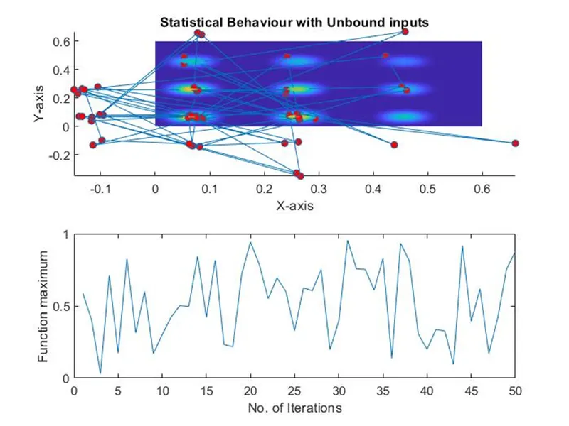
The random sampling of the genetic algorithm provides a new optimal value for the function every time the code is executed, as shown in the following plot. This, however, is consistent with the concept of Genetic Algorithm. The large number of red dots indicates that the values of the x and y co-ordinates change with each repetition.

case 2 :- Statistical Behaviour with upper and lower bounds.

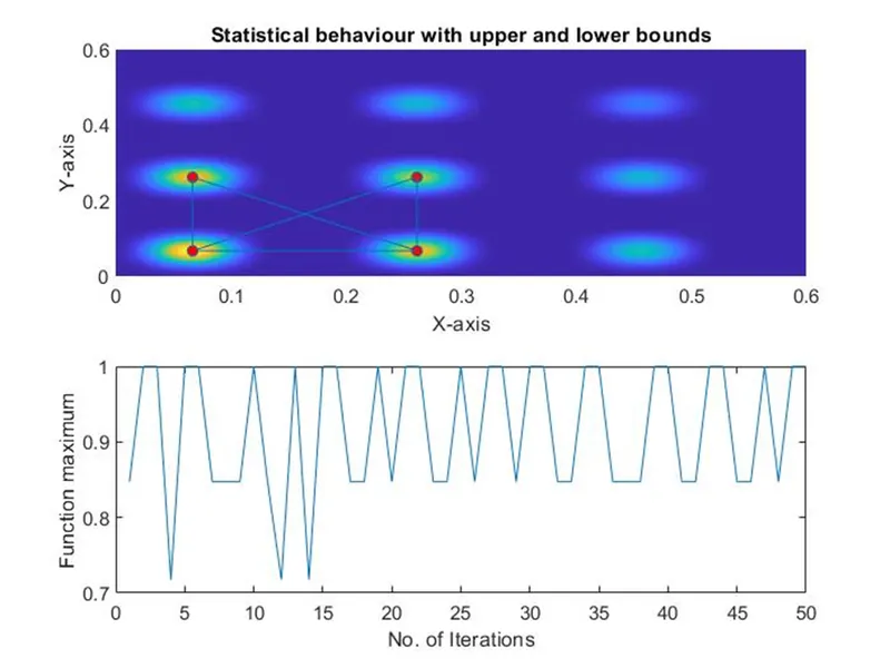
The convergence of x and y values may be seen in the given data. In comparison to the preceding figure, there are less red dots. This is the effect of giving the function higher and lower boundaries.

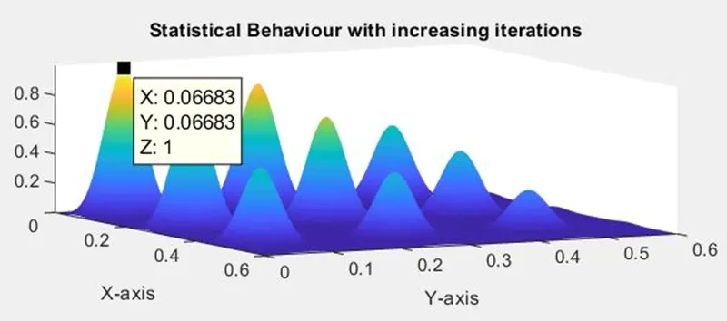
case 3 :- Statistical Behaviour with increasing iterations of GA.

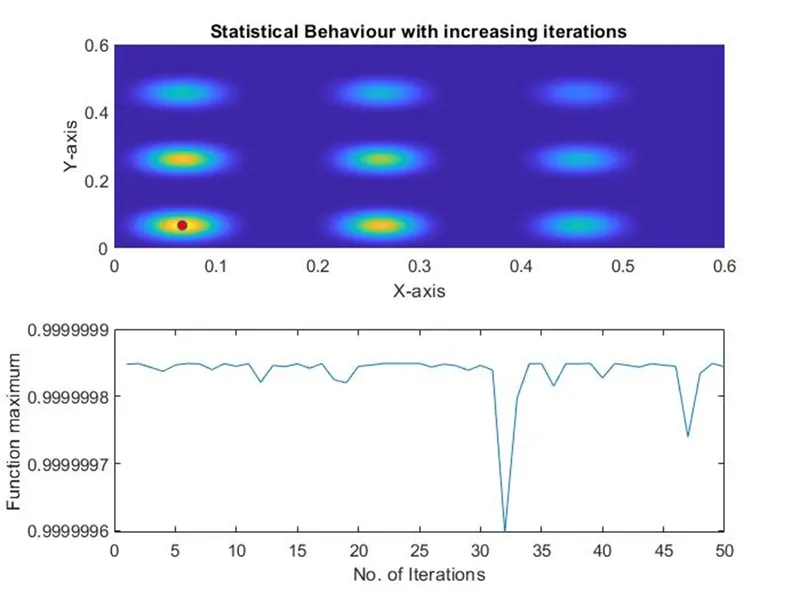
The number of iterations is raised to 300 in this study in order to converge and locate the function's global maxima. On the stalagmite function, we can see that there is just one red dot, which is the requisite global maximum point.

Errors:

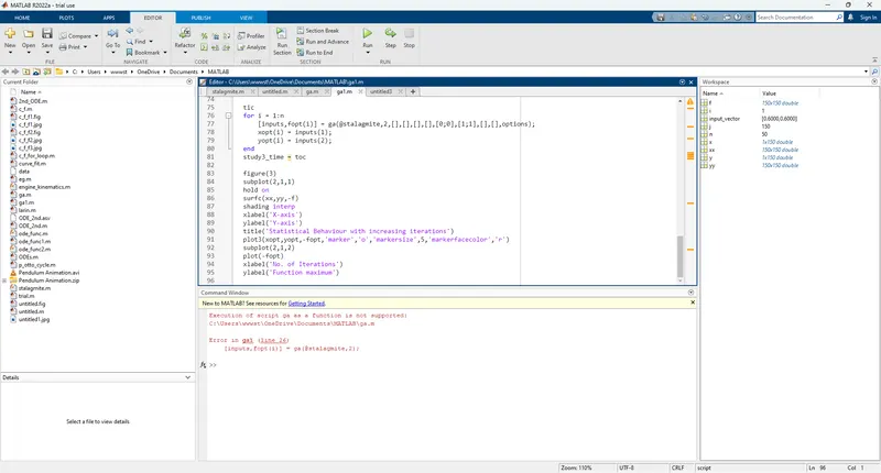
This is the major error i faced then i solved by replacing the function and runs one by one