Project 2 - Rankine cycle Simulator
Theory of Rankine Cycle – Equations and Calculation
Theory of Rankine Cycle
Theory:
The Rankine cycle was named after him and describes the performance of steam turbine systems, though the theoretical principle also applies to reciprocating engines such as steam locomotives. The Rankine cycle is an idealized thermodynamic cycle of a constant pressure heat engine that converts part of heat into mechanical work. In this cycle, the heat is supplied externally to a closed loop, which usually uses water (in a liquid and vapor phase) as the working fluid. In contrast to the Brayton cycle, the working fluid in the Rankine cycle undergo the phase change from a liquid to vapor phase and vice versa.
While many substances could be used as the working fluid in the Rankine cycle (inorganic or even organic), water is usually the fluid of choice due to its favorable properties, such as its non-toxic and unreactive chemistry, abundance, and low cost, as well as its thermodynamic properties. For example, water has the highest specific heat of any common substance – 4.19 kJ/kg K. Moreover it has a very high heat of vaporization, making it an effective coolant and medium in thermal power plants and other energy industries. In the case of the Rankine cycle, the Ideal Gas Law almost cannot be used (steam does not follow pV=nRT). Therefore all important parameters of water and steam are tabulated in so-called “Steam Tables”.
One of the major advantages of the Rankine cycle is that the compression process in the pump takes place on a liquid. By condensing the working steam to a liquid (inside a condenser), the pressure at the turbine outlet is lowered, and the energy required by the feed pump consumes only 1% to 3% of the turbine output power. These factors contribute to higher efficiency for the cycle.
In an ideal Rankine cycle, the system executing the cycle undergoes a series of four processes: two isentropic (reversible adiabatic) processes alternated with two isobaric processes:
Rankine Cycle – Diagram
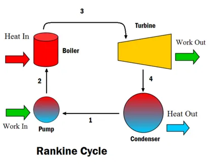
Isentropic compression (compression in centrifugal pumps) – The liquid condensate is compressed adiabatically from state 1 to state 2 by centrifugal pumps (usually by condensate pumps and then by feedwater pumps). The liquid condensate is pumped from the condenser into the higher-pressure boiler. In this process, the surroundings work on the fluid, increasing its enthalpy (h = u+pv) and compressing it (increasing its pressure). On the other hand, the entropy remains unchanged. The work required for the compressor is given by WPumps = H2 – H1.
Isobaric heat addition (in a heat exchanger – boiler) – In this phase (between state 2 and state 3), there is a constant-pressure heat transfer to the liquid condensate from an external source since the chamber is open to flow in and out. The feedwater (secondary circuit) is heated to the boiling point (2 → 3a) of that fluid and then evaporated in the boiler (3a → 3). The net heat added is given by Qadd = H3 – H2
Isentropic expansion (expansion in a steam turbine) – Steam from the boiler expands adiabatically from state 3 to state 4 in a steam turbine to produce work and then is discharged to the condenser (partially condensed). The steam works on the surroundings (blades of the turbine) and loses an amount of enthalpy equal to the work that leaves the system. The work done by the turbine is given by WT = H4 – H3. Again, the entropy remains unchanged.
Isobaric heat rejection (in a heat exchanger) – In this phase, the cycle completes by a constant-pressure process in which heat is rejected from the partially condensed steam. There is heat transfer from the vapor to cooling water flowing in a cooling circuit. The vapor condenses, and the temperature of the cooling water increases. The net heat rejected is given by Qre = H4 – H1
During a Rankine cycle, the pumps’ work is done on the fluid between states 1 and 2 (isentropic compression). Work is done by the fluid in the turbine between stages 3 and 4 (isentropic expansion). The difference between the work done by the fluid and the work done on the fluid is the network produced by the cycle, and it corresponds to the area enclosed by the cycle curve (in the pV diagram). The working fluid in a Rankine cycle follows a closed loop and is reused constantly.
As can be seen, it is convenient to use enthalpy and the first law in terms of enthalpy to analyze this thermodynamic cycle. This form of the law simplifies the description of energy transfer. At constant pressure, the enthalpy change equals the energy transferred from the environment through heating:
Isobaric process (Vdp = 0):
dH = dQ → Q = H2 – H1
At constant entropy, i.e., in isentropic process, the enthalpy change equals the flow process work done on or by the system:
Isentropic process (dQ = 0):
dH = Vdp → W = H2 – H1
Code
clear all
close all
clc

% Rankine Cycle Simulator ouputes

fprintf(' Rankine Cycle \n')
fprintf(' 1-2 is Isentropic Expansion in Turbine \n')
fprintf(' 2-3 is constant pressure heat removal \n')
fprintf(' 3-4 is Isentropic Compression in Pump \n')
fprintf(' 4-1 is Constant pressure Heat addition in Boiler \n')

% Inputes
p1 = 30;        %Turbine inlet pressure
T1 = 400;       %Turbine inlet temprature
p2 = 0.05;      %Condenser inlet pressure or Tubrbine outlet pressure

% Using Xsteam file for State point 1
h1 = XSteam('h_pT', p1, T1);        % Enthaply at pressure and Temprature 1
s1 = XSteam('s_pT', p1, T1);        % Entropy at pressure and Temprature 1

% Using Xsteam file for State point 2
s2 = s1;                            % Because of Isentropic Expansion
sf2 = XSteam('sL_p', p2);           % Saturated liquid entropy at pressure 2
sg2 = XSteam('sV_p', p2);           % Saturated vapour entropy at pressure 2
x2 = (s2-sf2)/(sg2-sf2);            % Vapour Fraction at point 2
hf2 = XSteam('hL_p', p2);           % Saturated liquid Enthalpy at pressure 2
hg2 = XSteam('hV_p', p2);           % Saturated vapour Enthalpy at pressure 2
h2 = hf2 + (x2*(hg2-hf2));          % Enthalpy at state point 2

% Using Xsteam file for State point 3
p3 = p2;                            % Constant Pressure heat removal process
s3 = Xsteam('sL_p', p3);            % Saturated liquid entropy at Pressure 3
h3 = XSteam('hL_p', p3);            % Saturated liquid Enthalpy at Pressure 3

% Using Xsteam file for State point 4
s4 = s3;                            % Isentropic Compression process
p4 = p1;                            % Constant Pressure heat rejection

% Work done in Turbine for the rankine cycle
W_T = h1-h2;

% Work done for PUMP
v3 = XSteam('vL_p',p3);         % Saturated Liquid Vapour at pressure 3
W_P = v3*(p4-p3)*100;           % Work done for pump
h4 = h3 - W_P;                  % Enthalpy at point 4

% Net work done for Rankine Cycle
W_net = W_T - W_P;

% Heat Addition to System
Q_in = h1-h4;

% Heat Rejection from System
Q_out = h2-h3;

% Thermal Efficiency of Rankine Cycle
T_eff = (W_net/Q_in)*100;

%specific steam consumption  = (Mass flow rate / Net work done)
Sp_S = (3600/W_net);

% Calculation of Temperature at All state Point 2, 3 and 4
T3 = XSteam('Tsat_p',p3);           % Saturation Temperature at Pressure 3
T2 = T3;                            % Becuase of Constant Pressure Heat addition
Cp4 = XSteam('Cp_ps',p4,s4);        % Specific isobaric heat capacity
Cv4 = XSteam('Cv_ps',p4,s4);        % Specific isochoric heat capacity
k = Cp4/Cv4;
T4 = T3/((p3/p4)^((k-1)/k));        % Temperature at State point 4

% Calculation of Other constant for saturated liquid and Vapour
T6 = XSteam('Tsat_p', p1);          % Saturated Temperature at Pressure 1
s5 = XSteam('sL_p', p1);            % Saturated Liquid entropy at pressure 1
s6 = XSteam('sV_p', p1);            % Saturated Vapour entropy at Pressure 1
h5 = XSteam('hL_p', p1);            % Saturated Liquid Enthalpy at Pressure 1
h6 = XSteam('hV_p', p1);            % Saturated Vapour Enthalpy at pressure 1
T5 = T6;

%Plotting for Saturation Line
T = linspace(1,560,1000);
for i = 1:length(T)
    sf(i) = XSteam('sL_T' ,T(i));   % Saturated Liquid Entropy
    sg(i) = XSteam('sV_T' ,T(i));   % Saturated Vapour Entropy
    hf(i) = XSteam('hL_T' ,T(i));   % Saturated Liquid Enthalpy
    hg(i) = XSteam('hV_T' ,T(i));   % Saturated Vapour Enthalpy

end

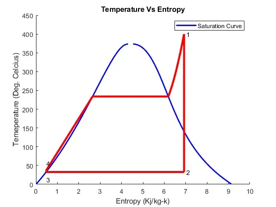
% Plotting T-S Diagram for Rankine Cycle
figure(1)
hold on
plot(sf,T,'color','b','linewidth',2)
plot(sg,T,'color','b','linewidth',2)
plot([s1 s2],[T1 T2], 'color', 'r', 'linewidth',3)
plot([s2 s3],[T2 T3], 'color', 'r', 'linewidth',3)
plot([s3 s4],[T3 T4], 'color', 'r', 'linewidth',3)
plot([s4 s5],[T4 T5], 'color', 'r', 'linewidth',3)
plot([s5 s6],[T5 T6], 'color', 'r', 'linewidth',3)
s_1 = linspace(s6,s1,1000);
for j = 1:length(s_1)
    Tc(j) = XSteam('T_ps',p1,s_1(j));
end

plot(s_1,Tc,'color','r','linewidth',3)
text(s1+0.1, T1, '1')
text(s2+0.1, T2, '2')
text(s3, T3-20, '3')
text(s4, T4+20, '4')
title('Temperature Vs Entropy')
xlabel('Entropy (Kj/kg-k)')
ylabel('Temeperature (Deg. Celcius)')
legend('Saturation Curve')

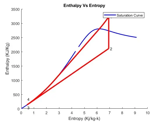
% Plotting H-S Diagram for Rankine Cycle
figure(2)
hold on
plot(sf,hf,'color','b','linewidth',2)
plot(sg,hg,'color','b','linewidth',2)
plot([s1 s2],[h1 h2],'color','r','linewidth',3)
plot([s2 s3],[h2 h3],'color','r','linewidth',3)
plot([s3 s4],[h3 h4],'color','r','linewidth',3)
hc = linspace(h4,h5,100);
for k = 1:length(hc)
    s_c(k) = XSteam('s_ph',p1,hc(k));
end
plot(s_c,hc,'color','r','linewidth',3)
plot([s5 s6],[h5 h6],'color','r','linewidth',3)
for l = 1:length(s_1)
    h_c(l) = XSteam('h_ps',p1,s_1(l));
end
plot(s_1,h_c,'color','r','linewidth',3)
text(s1+0.1,h1,'1')
text(s2+0.1,h2,'2')
text(s3,h3-100,'3')
text(s4,h4+200,'4')
title('Enthalpy Vs Entropy')
xlabel('Entropy (Kj/kg-k)')
ylabel('Enthalpy (KJ/Kg)')
legend('Saturation Curve')

% Displaying Results in Command window
disp('Results of Rankine Cycle')
%At state point 1
fprintf('At state point 1 \n')
fprintf('P1 = %10f in Bar \n',p1);
fprintf('T1 = %11f in Deg.Celcius \n',T1);
fprintf('H1 = %12f in KJ/Kg \n',h1);
fprintf('S1 = %9f in KJ/Kg-k \n',s1);

%At state point 2
fprintf('At state Point 2 \n')
fprintf('P2 = %10f in Bar \n',p2);
fprintf('T2 = %11f in Deg.Celcius \n',T2);
fprintf('H2 = %12f in KJ/Kg \n',h2);
fprintf('S2 = %9f in KJ/Kg-k \n',s2);

%At state point 3
fprintf('At state point 3 \n')
fprintf('P3 = %10f in Bar \n',p3);
fprintf('T3 = %11f in Deg.Celcius \n',T3);
fprintf('H3 = %12f in KJ/Kg \n',h3);
fprintf('H3 = %12f in KJ/Kg \n',h3);
fprintf('S3 = %9f in KJ/Kg-k \n',s3);

%At state point 4
fprintf('At state Point 4 \n')
fprintf('P4 = %10f in Bar \n',p4);
fprintf('T4 = %11f in Deg.Celcius \n',T4);
fprintf('H4 = %12f in KJ/Kg \n',h4);
fprintf('S4 = %9f in KJ/Kg-k \n',s4);

fprintf('Turbine Work Done = %14f in KJ/Kgn \n',W_T)
fprintf('Pump Work Done = %15f in KJ/Kg \n',W_P)
fprintf('Net Work Done  = %17f in KJ/Kg \n',W_net)
fprintf('Thermal Efficiency = %13f in percentage \n',T_eff)
fprintf('Sp. Steam Consumption = %f in KJ/Kw \n',Sp_S)
Code explanation
the line by line explanation is added in the program only
Results
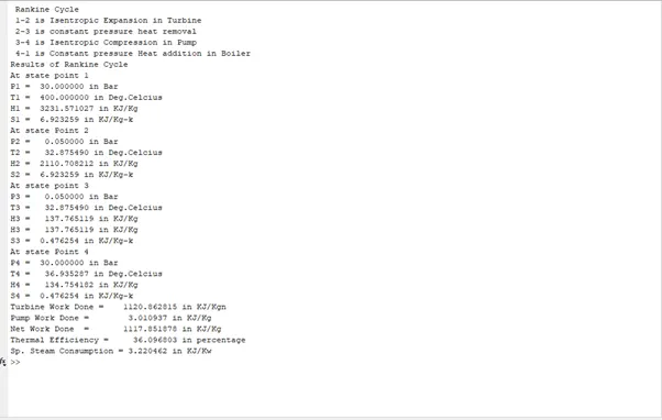
Command window
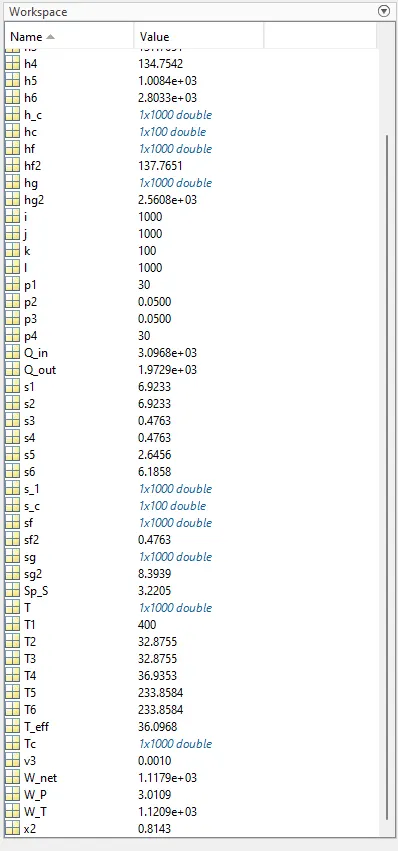
Workspace
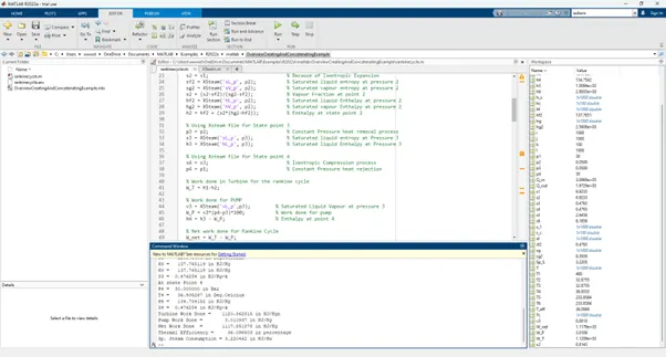
Graphs
Errors Faced
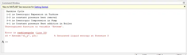
This error I cleared by correcting the spelling
Only this error if faced. there are no such major errors while programming
References
https://www.sciencedirect.com/topics/engineering/back-work-ratio
https://en.wikipedia.org/wiki/Rankine_cycle
https://energyeducation.ca/encyclopedia/Rankine_cycle
https://www.electrical4u.com/ideal-verses-actual-in-rankine-cycle/