Week 3 - Solving second order ODEs

Solving the second order ODEs

Aim: Using ODE determine the transient behaviour of a system. taking example as a simple pendulum

Objective: Our objective is to write a program that solves the following ODE. This ODE represents the equation of motion of a simple pendulum with damping

Theory: The way the pendulum moves depends on the Newtons second law. When this law is written down, we get a second order Ordinary Differential Equation that describes the position of the "ball" w.r.t time. Similarly, there are hundreds of ODEs that describe key phenomena and if you have the ability to solve these equations then you will be able to simulate any of these systems.

Procedure:

In the above equation

In the above equation,

g = gravity in m/s2,

L = length of the pendulum in m,

m = mass of the ball in kg,

b=damping coefficient.

values,

L=1 metre,

m=1 kg,

b=0.05.

g=9.81 m/s2.

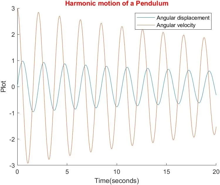
We are Simulating the motion between 0-20 sec, for angular displacement=0, angular velocity=3 rad/sec at time t=0.

program

% Objective: Solving second order ODEs of a penedulum


clear all
close all
clc

b = 0.05
g = 9.81 
l = 1 
m = 1

% initial condition
% angular displacement is 0 and angular velocity is 3

theta_0 = [0;3]

% Pendulum oscillates between 0-20 seconds

t_span = linspace(0,20,600)

% solving ODE
[t,results] = ode45(@(t,theta) ode_func(t, theta, b,g,l,m), t_span, theta_0);

%Plotting
figure(1)
hold on
plot(t,results(:,1))
plot(t,results(:,2))
title('Harmonic motion of a Pendulum',Color='r')
legend('Angular displacement', 'Angular velocity')
ylabel('Plot')
xlabel('Time(seconds)')

ct =1;
 for i = 1:length(results(:,1))
 x_start = 0     
 y_start = 0
 x_end = l*sin(results(i,1))
 y_end = -l*cos(results(i,1))
 
 % plotting for the movie
 figure(2)
 plot([-1 1], [0 0], 'linewidth', 5)
 hold on
 plot([x_start x_end],[y_start y_end],'linewidth',3)
 hold on
 
 plot(x_end,y_end,'o','markersize',30,'markerFacecolor','g')
 title('Pendulum Animation')
 axis([-1.5 1.5 -1.5 1])
 pause(0.03)
 hold off 
 
 M(ct) = getframe(gcf)
 ct = ct+1
 
 end
 
 
% Movie

 movie(M)
videofile=VideoWriter('Pendulum Animation.avi', 'uncompressed avi')
open(videofile)
writeVideo(videofile,M)
close(videofile)

Main program to solve ODE

%  function program or main program to solve the
% ODE


function [dtheta_dt] = ode_func1(t,theta,b,g,l,m);

theta1= theta(1);
theta2= theta(2);
dtheta1_dt = theta2;
dtheta2_dt = -(b/m)*theta2 - (g/l)*sin(theta1);
dtheta_dt = [dtheta1_dt; dtheta2_dt];
end 

Program explanation

Close all, clear all, clc are used to close all figures, clean workspace, clean command window. Giving the values for b, g, l, m as mentioned above. we are going to give the initial conditions as angular displacement is 0 and angular velocity as 3

Theta_0 = [angular displacement; angular velocity]

And pendulum oscillating between 0-20 seconds

t_span = linspace(0,20,600)

solving the equation as mentioned above using ode45

here I am mentioning an example for ode45 function

eg: Solve the ODE using the ode45 function on the time interval [0 20] with initial values [2 0]. The resulting output is a column vector of time points t and a solution array y. Each row in y corresponds to a time returned in the corresponding row of t. The first column of y corresponds to y1, and the second column corresponds to y2.

[t,y] = ode45(@vdp1,[0 20],[2; 0]);

Separately we are plotting all the graphs and making it as a movie using getframe

movie(M)

videofile=VideoWriter('Pendulum Animation.avi', 'uncompressed avi')

open(videofile)

writeVideo(videofile,M)

close(videofile)

Results:

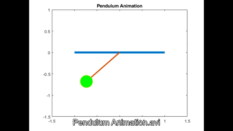
https://drive.google.com/file/d/1TdF7KyIYfAbKiV3yvkpIZjr-iL53Mzc7/view?usp=sharing

the above link include the pendulum video . its as a zip format extract and see

Error faced

There is not such an error faced while programming only small mistakes like semicolon, error in some commands and spelling mistakes while doing movie command

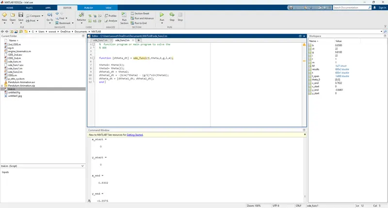
Those errors are solved by seeing the command window