Week 4.1 - Genetic Algorithm

Genetic Algorithm (GA) is a technique for solving both constrained and unconstrained optimization problem. It is based on the theory of natural selection . it constantly alter the population size to reach to an ultimate minima.

Phases of genetic algorithm

Phase 1- Initializing population

The code generates its random population of defined size and from that it evaluates the fitness of the members of the population according to which it forms new population baased on no. of iterations performed .

Phase 2 - Fitness Function

It is the function which we have to optimize which is done with the help of numbers of generations which have been formed by the code accordance with the fitness values of each member generated

Phase 3 - Selection

This phase selects the fittest individuals and let them pass there genes to the next generation . The main goal of this phase is to find the region where the chance of getting the best solutions are more .

Phase 4 - Reproduction

It happens by two methods Mutation & Crossover

Syntax of GA

x= ga(function, nvars)

finds a local unconstrained minima of 'function' where nvars is the no of designated variables

x= ga(func,nvars,A,b,Aeq,Beq,lb,ub)

this function generates the minima bounded by lb and ub

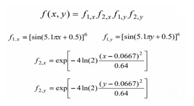
In this program we need to find the maxima of the stalagmite function so we use -fopt in the output to get the maxima .

Main Program

x = linspace(0,0.6,150);
y= linspace(0,0.6,150);
[X,Y]=meshgrid(x,y);
%create the mesh grid out of the X & Y 

%Run the stalagmite function 
num_cases= 150;
for i=1:length(X)
    for j=1:length(Y)
        input_vector(1)=X(i,j);
        input_vector(2)=Y(i,j);
        f(i,j)=stalagmite(input_vector);
    end
end

surfc(X,Y,-f); %generating the surface

shading interp %To remove the lines produced by the mesh grid

tic
%to count the calculation time 


%calling the GA function to optimize the stalagmite function 
for i=1:num_cases

[inputs,fopt(i)]=ga(@stalagmite,2); %calculating the optimized value of the function

xopt(i)=inputs(1); %at each iteration

yopt(i)=inputs(2);

end


% PLOTING THE GRAPH

figure(1)

subplot(2,1,1)

surfc(X,Y,-f);

hold on
%plotting the line graph over the surface graph 

shading interp

plot3 (xopt,yopt,(-fopt),'marker','o','markersize',5,'markerfacecolor','r');

xlabel('x');

ylabel('y');



subplot(2,1,2)

plot(-fopt);

xlabel('iterations')

ylabel('function min value')
study1_time = toc

% STATISTICAL BEHAVIOUR (UNBOUNDED)

tic %calculating the study time through tic and toc command

for i=1:num_cases

[inputs,fopt(i)]=ga(@stalagmite,2);
%calculating the optimized value of the function

xopt(i)=inputs(1); %at each iteration

yopt(i)=inputs(2);

end

study2_time = toc 
%displaying the time taken to evaluate

% PLOTING THE GRAPH

figure(2)

subplot(2,1,1)

surfc(X,Y,-f);

hold on

shading interp

plot3(xopt,yopt,-fopt,'marker','o','markersize',5,'markerfacecolor','r');

xlabel('x');

ylabel('y');

grid on

subplot(2,1,2)

plot(-fopt)

xlabel('iterations')

ylabel('function min value')


% STATISTICAL BEHAVIOUR (BOUNDED

tic %calculating the study time through tic and toc command

for j=1:num_cases

[inputs,fopt(j)]=ga(@stalagmite,2,[],[],[],[],[0;0],[1;1]); %calculating the optimized value of the function

xopt(j)=inputs(1); %at each iteration with boundation

yopt(j)=inputs(2);

end

study3_time=toc

%PLOTTING

figure(3)

subplot(2,1,1)

hold on

surfc(X,Y,-f)

shading interp

plot3(xopt,yopt,-fopt,'marker','o','markersize',5,'markerfacecolor','r');

xlabel('x');

ylabel('y');

grid on

subplot(2,1,2)

plot(-fopt);

xlabel('iterations')

ylabel('function min value')

Stalagmite function

function [f] = stalagmite(input_vector)

x = input_vector(1);

y = input_vector(2);

f1_x = (sin(5.1*pi*x + 0.5)).^6;

f1_y = (sin(5.1*pi*y + 0.5)).^6;

t1 = ((x-0.0667).^2)/(0.64);

f2_x = exp(-4.*log(2)*t1);

t2 = ((y-0.0667).^2)/(0.64);

f2_y = exp(-4.*log(2)*t2);

f = -(f1_x.*f2_x.*f1_y.*f2_y);

end

step 1 - create the mesh-grid of X Y

step 2 - run the stalegmite function by creating input vectors

step 3 - generate the surface graph

step 4 - obtain the optimized value in xopt and yopt.

step 5- generate the 3d line line graph for optimized value and functional value.

step 6 - generate the (-fopt) vs iterations graph

repeat the same for unconstrained GA and bounded GA optimization

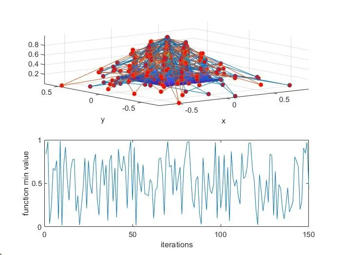
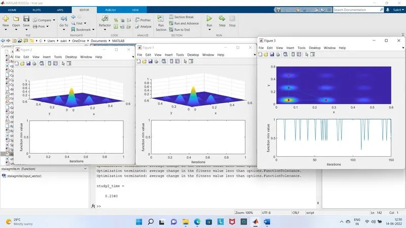
case 1 unconstrained optimization

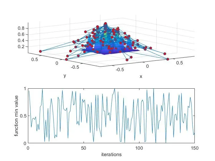
case 2 unconstrained optimization

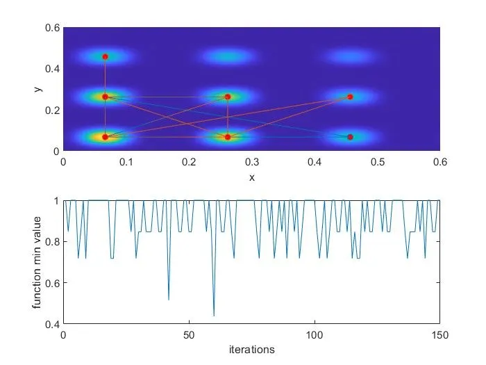
case 3 - constrained optimization

error faced during programming -

logical error in stalagmite function

fopt value was coming infinity .