Week 3 - Solving second order ODEs

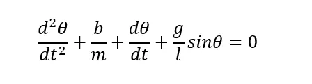
The motion of a damped simple pendulum is governed by the equation

Main Program

clear all
close all
clc
b=0.05;
g=9.81;
l=1.00;
m=1;

theta_0=[0,3];
t_span = linspace(0,20,300);

[t, results]= ode45(@(t,theta) ode_func(t,theta,b,g,l,m),t_span,theta_0);
figure(1)
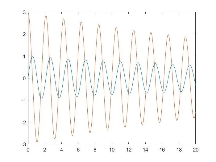
plot (t,results(:,1));
hold on;
plot (t,results(:,2));

figure(2)
ct=1;
l1=0.5;
for i=1:length(results(:,1))
    x0=0;
    y0=3;
    x1=l1*sin(results(i,1));
    y1=-l1*cos(results(i,1));
plot([1,-1],[3 3])
hold on 
plot([x0 x1],[y0 y1],'LineWidth',4,'Color','b');
axis=[-5 1.5 -1.5 1.5];
plot (x1,y1,'O','MarkerSize',20,'Color','r');
pause(0.0001);
M(ct)=getframe(gcf);
hold off
ct=ct+1;
end
movie(M)
videofile=VideoWriter('simple_pendulum.avi');
open(videofile);
writeVideo(videofile,M);
close(videofile);

Function

function [dtheta_dt]= ode_func(t,theta,b,g,l,m)
theta1=theta(1);
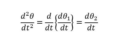
theta2=theta(2);
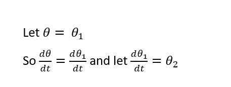
dtheta1_dt=theta2;
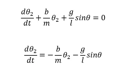
dtheta2_dt= -(b/m)*theta2-(g/l)*sin(theta1);
dtheta_dt=[dtheta1_dt;dtheta2_dt];

end

Step 1

Declare all the provided constants for the solutions

Step 2

Declare the intial conditon at 0 displacement point.

Step 3

Call the ODE funciton and with all the required arguements

Step4

Plot the graph of both displacement and velocity on same graph using the hold on command

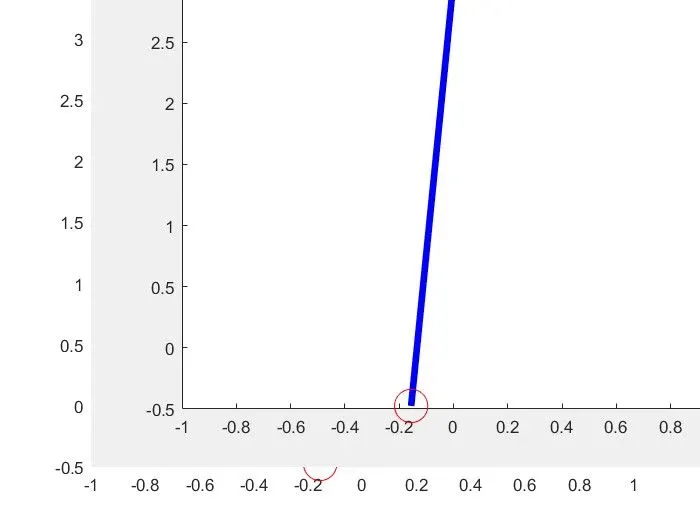
Create the animation

Step5

Create the movie out of the scenes.

https://youtu.be/01p2IYrZD-0