Week 4.1 - Genetic Algorithm

• Write a code in MATLAB to optimise the stalagmite function and find the global maxima of the function.
• Plot graphs for all 3 studies and for F maximum vs no. of iterations. Title and axes labels are a must, legends could be shown if necessary.
• Step-wise explanation of your code.

A stalagmite function generally refers to the function with which we are generating values over a stalagmite kind of surface for finding out the local and global maxima and minima of that particular given function.

stalagmite function is defined separately and later it is called in GA main program.

stalagmite function is defined as below

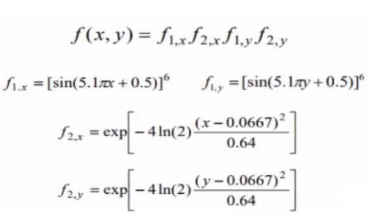
Stalagmite function:

% creating a stalagmite program
function [v] = stalagmite_one(input_vector)

x=input_vector(1);
y=input_vector(2);

f1x = (sin((5.1*pi).*x+0.5)).^6;
f1y = (sin((5.1*pi).*y+0.5)).^6;
f2x = exp(((x-0.0667).^2/0.64).*(-4*log(2)));
f2y = exp(((y-0.0667).^2/0.64).*(-4*log(2)));

v = -(f1x*f2x*f1y*f2y);

end

• Creating the Stalagmite_one function by passing the input_vectoras the argument for the variable x and y.The output of the function is stored in the variable [v]
• The input_vector(1) is stored in the variable x
• The input_vector(2) is stored in the variable y
• f1x,f1y,f2x,f2y are defined as per the stalagmite equation
• Now v= -(f1x*f2x,f1y,f2y) is calculated and negative sign is given to the equation so as to obtain global maxima.

Coding for main GA program:

1st iteration:

• start the program with clear all,close all and clc
• using linspace command we define x and y variable
• Now num_cases is used to run the program(no.of times) 50 times to evaluate the results.
• The input vectors are transformed into variable array [xx,yy] to evaluate x and y variables to plot 3 dimensional suface plots.
• To assign the values to the variables now 2 for loops are used. With this we can get the value of stalagmite function(code which already defined above) at the various values of x and y.
• Now GA is made to run for 3 iterations
• study 1 is statistical behaviour
• tic and toc command is used to calculate the total study time at the start and the end of the for loop in each study.
• now calling a for loop from 1:num_cases using variable "i".
• Genetic algorithm (ga) is a solver which pass the function to the solve the stalagmite_one with the 2 variables x and y
• inputs , fopt(i) are the output of GA.
• fopt(i) is the output to store the optimum values of stalagmite_one for all the values of x and y
• Inputs are the output to store the optimum values if the valariable of stalagmite_one as selected
• The value of x is saved in xopt(i) and y value in yopt(i) in every iteration of for loop.
• Now plot is generated by using figure(1) and by selecting subplot
• Now holdon command is used to retain the plots in current axes so that new plots added to the axes does not delete the existing plots
• Now surfc command is used to create surface plots of the values of stalagmite function which is stored in -f.
• Now 3D plot is generated using plot3 command
• Now title , x label and y label are provided.
• Subplot 2 is selected and -fopt is plotted using the plot command.

clear all
close all
clc

x=linspace(0,0.6,150);
y=linspace(0,0.6,150);

num_cases=50
% evaluating the stalagmite function
[xx , yy] = meshgrid(x,y);
for i=1:length(xx)
    for j=1:length(yy)
        input_vector(1)=xx(i,j);
        input_vector(2)=yy(i,j);
        f(i,j) = stalagmite_one(input_vector);
      
    end
end

tic
%study 1-statistical behaviour
for i=1:num_cases;
    [inputs,fopt(i)]=ga(@stalagmite_one,2);
    xopt(i)=inputs(1);
    yopt(i)=inputs(2);
    
end
study1_time=toc
figure(1)
subplot(2,1,1)
hold on
surfc(x,y,-f)
plot3(xopt,yopt,-fopt,'marker','o','markersize',5,'markerfacecolor','r')
title('unbounded input')
subplot(2,1,2)
plot(-fopt)
xlabel('iterations')
ylabel('function minimum')

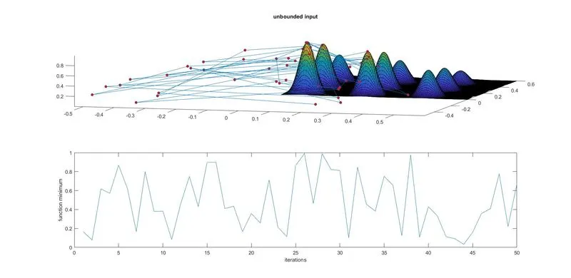
In the above plot we can see that the inputs are unbounded and GA has mapped local maxima points outside the stalagmite function and also we did not get a particular point with this graph and the study time observes as 5.2851

2nd iteration:

• study 2 statistical behaviour with upper and lower bound
• same like 1st iteration , the 2nd iteration is made to run with a for loop
• plot is generated by using figure (2) and same procedure is used to plot the 2nd iteration

tic
%study 2-statistical behaviour with upper and lower bound
for i=1:num_cases;
    [inputs,fopt(i)]=ga(@stalagmite_one,2,[],[],[],[],[0,0],[1,1]);
    xopt(i)=inputs(1);
    yopt(i)=inputs(2);
    
end
study2_time=toc
figure(2)
subplot(2,1,1)
hold on
surfc(x,y,-f)
shading interp
plot3(xopt,yopt,-fopt,'marker','o','markersize',5,'markerfacecolor','r')
title('bounded input')
subplot(2,1,2)
plot(-fopt)
xlabel('iterations')
ylabel('function minimum')

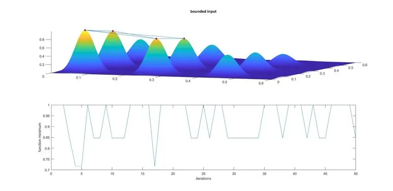
Now the plot is more clear and optimised compared to the 1st iteration and we could get the values within the range because in this study we have defined by bounds(upper and lower bound) . The study time observed as 5.9973

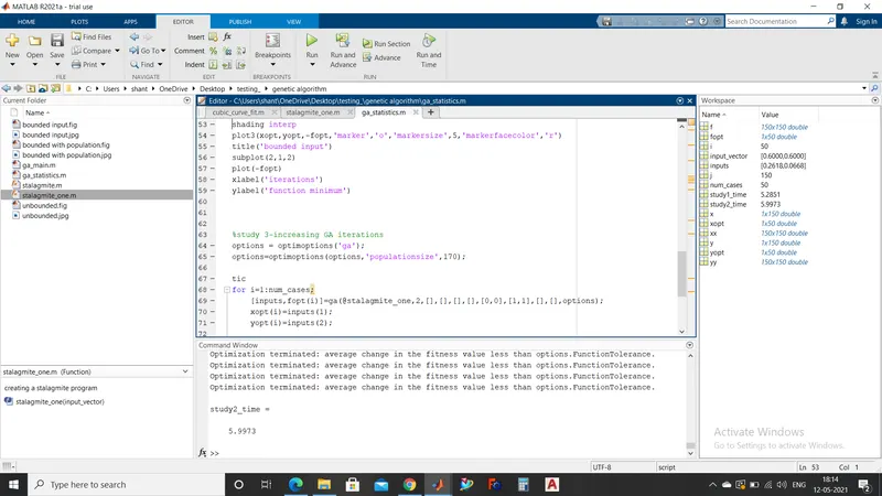
3rd iteration:

• The same procedure is followed
• But here we are increasing the GA iterations to 170
• Plot is generated by using the figure(3)

%study 3-increasing GA iterations
options = optimoptions('ga');
options=optimoptions(options,'populationsize',170);

tic
for i=1:num_cases;
    [inputs,fopt(i)]=ga(@stalagmite_one,2,[],[],[],[],[0,0],[1,1],[],[],options);
    xopt(i)=inputs(1);
    yopt(i)=inputs(2);
    
end
study3_time=toc
figure(3)
subplot(2,1,1)
hold on
surfc(x,y,-f)
shading interp
plot3(xopt,yopt,-fopt,'marker','o','markersize',5,'markerfacecolor','r')
title('bounded inputs with modified population size')
subplot(2,1,2)
plot(-fopt)
xlabel('iterations')
ylabel('function minimum')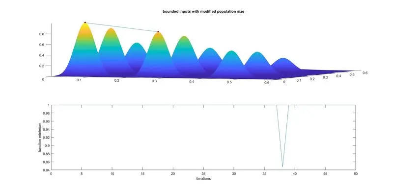

Now we could see the optimised value with accurate result. As the no. of iterations and population size is increased the study time is also more compared to previous 2 iterations . And we could get the global maxima with accurate result by increasing the no. of iteration with increasing population size

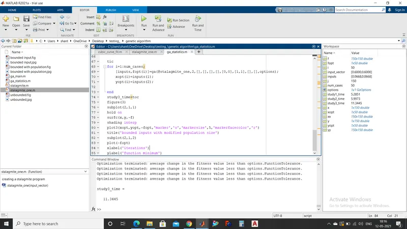
The study time observed in this iteration is 11.3445

• Clearly expalin the concept of genetic algorithm in your own words and also explain the syntax for ga in MATLAB in your report.

To perform the optimisation process we need to choose the optimisation technique . Genetic algorithm is one of theoptimisation process to get the better solution to a given problem.It is a search based algorithm which is based on the concept of natural selections and genetics.

The below flow chart describes the working of genetic algorithm to find the optimised solution.

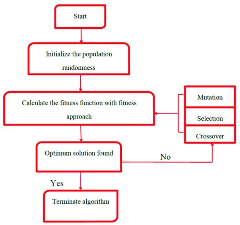
Genetic algorithms are commonly used to generate high-quality solutions to optimisation and search based problems by depending on biologically inspired operations such as selection,cross-over and mutation.

In GA we have a population of a possible solution i.e set of sample data to a given problem . These solution undergo reombination and mutation (as menioned above it undergoes natural process)and producing a childern. The same process is being repeated for various generations. Every individual is given a fitness value and fitter individual are given higher chance to mate and yield more fitter individuals.The process repeats till the optimum solution is found

This process is repeated over various generations till we reach a stopping criterion.

The 3 operations which involves genetics process are as follows

1.Selection : In this selection, parents are selected from the sample data points.The objective of this process is to mainly select the highy fit individuals.

2.Cross-over : 2 parents are selected for producing a child. There are many ways for cross over. one way of doing cross over is set of genes from parent A is combined with Parent B to create new offspring.

cross-over methods:

1.one-point crossover

2.Multi point crossover

3.Uniform crossover

4.Davis order crossover

3.Mutation: Mutation is performed to maintain the genetic diversity from one generation of a population of chromosome to another. If mutation is not performed,the chromosomes will become too similar to each other ,convergence takes place soon and results in local minima

Types of Mutation methods:

1.Bit flip mutation

2.Swap mutation

3.Inversion mutation

Syntax for GA

x = ga(fun,nvars,A,b,Aeq,beq,lb,ub,nonlcon,options)

x - local minima point

fun - function to be called(i.e stalagmite function)

nvars - no of variables used (in our case 2 variables x and y)

A and b - indicates linear inequality constraints

Aeq and beq - indicates linear equality constraints

lb and ub - indicates lower bound and upper bound (in 2nd iteration we used lb and ub syntax i.e ga(@stalagmite_one,2,[],[],[],[],[0,0],[1,1]) where we set lb and ub to [] as there is no bound exists)

nonlcon - gives a 2 vectors representing inequalities and equalities

options -used to perform additional operations like increasing populations. This s done with "optimoptions" (in the 3rd iteration we used options syntax i.e ga(@stalagmite_one,2,[],[],[],[],[0,0],[1,1],[],[],options) )

• Mention the errors while programming.
• Steps taken to overcome those errors.
• Screenshots showing errors thrown in command window.

while coding a stalagmite function , assigned input variables to stalagmite_one but when called into main GA function it was assigned to stalagmite function instead of stalagmite_one

The following screenshots shows the errors or mistakes faced while executing the program

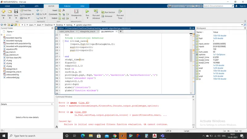
it is corrected by calling a function as stalagmite_one.

Results and conclusions:

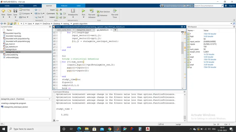
In the below image we can see the observed study time for all the 3 iterations and other calculated values in workspace