Week 4.1 - Genetic Algorithm
Defining Staligmate function for maxima:
%Defining Staligmate function for GA studies.

function [f_xy] = stalig(input_vec)
x = input_vec(1);
y = input_vec(2);
f_x1 = (sin(5.1*pi*x+0.5))^6;
f_y1 = (sin(5.1*pi*y+0.5))^6;
f_x2 = exp((-4*0.6931)*(x-0.0667)^2/0.64);
f_y2 = exp((-4*0.6931)*(y-0.0667)^2/0.64);

f_xy = -f_x1*f_y1*f_x2*f_y2; %Output is multiplied with -1 so that maxima can be alter to minima
end
Main Code for the genetic algorithm studies:
clear all
close all
clc

x = linspace(0, 0.6, 150);
y = linspace(0, 0.6, 150);

%Defining Mesh Grid for 2D array
[xx, yy] = meshgrid(x, y);

%staligmate call for output data collection of function
for i = 1:length(xx)
   for j = 1:length(yy)
     input_vec(1)=xx(i,j);
     input_vec(2)=yy(i,j);
     f(i,j)= stalig(input_vec);
   end
end
iteration = 70; %Number of iterations

%GA Study-1, Unbounded ga(fun,nvars)

for k = 1:iteration
   [input f_op(k)] = ga(@stalig,2);
   x_op(k) = input(1);
   y_op(k) = input(2);
end
%Result
maxima = -stalig(input);
disp(['Maxima of function (f) = ',num2str(maxima)]);
disp(['X-coordinate = ',num2str(input(1))]);
disp(['y-coordinate = ',num2str(input(2))]);

%Plot-1
figure(1);
subplot(2,1,1);
surfc(x, y, -f); %-f to reverse the output, so that the maximum can be visualised
colorbar;
shading interp;
hold on;
plot3(x_op, y_op, -f_op, 'Marker','*','MarkerSize',5,'color',[0.7 0.1 0.4]);
xlabel('x-coordinate[x]'); ylabel('y-coordinate[y]'); zlabel('output[f]');
hold off;
subplot(2,1,2);
plot(-f_op);
xlabel('Itration'); ylabel('Maxima')
grid on;


%GA Study-2, bounded; ga(fun,nvars,A,b,Aeq,beq,lb,ub)
%lower bound x=0 y=0; upper bound x=0.6 y=0.6

for k = 1:iteration
   [input, f_op(k)] = ga(@stalig,2,[],[],[],[],[0,0],[0.6,0.6]);
   x_op(k) = input(1);
   y_op(k) = input(2);
end

%Result
maxima = -stalig(input);
disp(['Maxima of function (f) = ',num2str(maxima)]);
disp(['X-coordinate = ',num2str(input(1))]);
disp(['y-coordinate = ',num2str(input(2))]);

%plot-2
figure(2);
subplot(2,1,1);
surfc(x, y, -f); %-f to reverse the output, so that the maximum can be visualised
colorbar;
shading interp;
hold on;
plot3(x_op, y_op, -f_op, 'Marker','*','MarkerSize',2,'color',[0.7 0.1 0.4]);
xlabel('x-coordinate[x]'); ylabel('y-coordinate[y]'); zlabel('output[f]');
hold off;
subplot(2,1,2);
plot(-f_op);
xlabel('Itration'); ylabel('Maxima')
grid on;

%GA Study-3,ga(fun,nvars,A,b,Aeq,beq,lb,ub,nonlcon,options)
%lower bound x=0 y=0; upper bound x=0.6 y=0.6
%initial population rise to 300
options = optimoptions('ga','PopulationSize',300);

for k = 1:iteration
   [input, f_op(k)] = ga(@stalig,2,[],[],[],[],[0,0],[0.6,0.6],[],options);
   x_op(k) = input(1);
   y_op(k) = input(2);
end
%Result
maxima = -stalig(input);
disp(['Maxima of function (f) = ',num2str(maxima)]);
disp(['X-coordinate = ',num2str(input(1))]);
disp(['y-coordinate = ',num2str(input(2))]);

%plot-3
figure(3);
subplot(2,1,1);
surfc(x, y, -f); %-f to reverse the output, so that the maximum can be visualised
colorbar;
shading interp;
hold on;
plot3(x_op, y_op, -f_op, 'Marker','*','MarkerSize',2,'color',[0.7 0.1 0.4]);
xlabel('x-coordinate[x]'); ylabel('y-coordinate[y]'); zlabel('output[f]');
hold off;
subplot(2,1,2);
plot(-f_op,'linewidth',2);
xlabel('Itration'); ylabel('Maxima')
axis([0 70 0.99 1])
grid on;
Results:
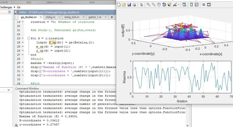
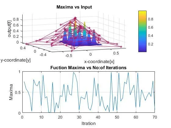
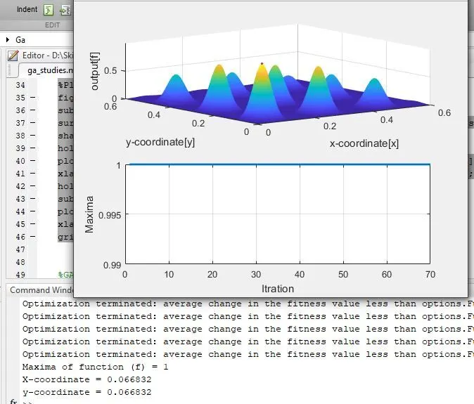
Study-1
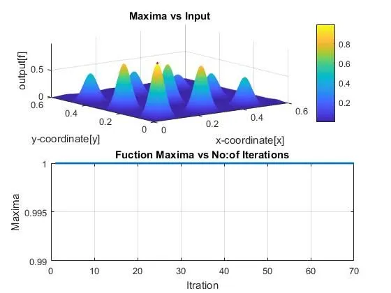
Study-2
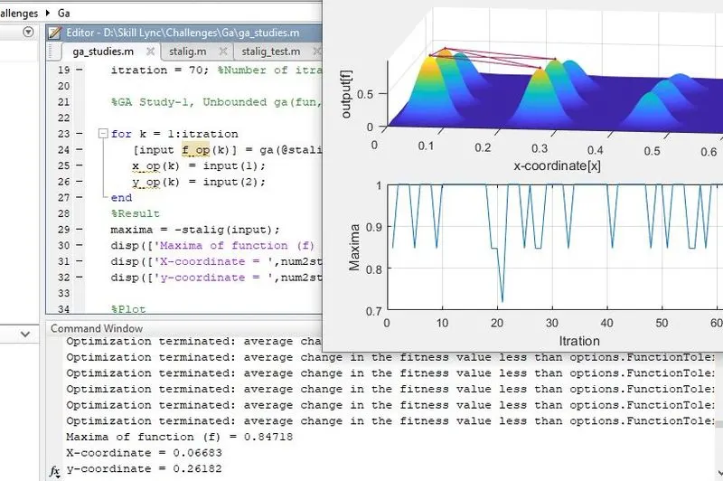
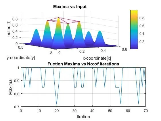
After defining the lower and upper bound.
Study-3
After defining the lower and upper bound, and increasing the initial sample size.
Genetic Algorithm:
A genetic algorithm is a method of solving optimization-related problems based on evolution theory very much related to biological evolution. The process starts with sample data point selection. The selection is based on a random function. The selected initial population then undergoes some process so that some elite is selected to produce a new generation. Each individual in a population is called a chromosome and the new individuals in the next population are called offspring
The process of selecting the parent chromosome is based on the following step by steps,
- Initial population and Fitness Value: The initial population selected by random function is ranked by fitness value or fitness points.
- Selection and expectation values: Now based on the fitness score a range of values are determined. These values are known as expectation values. Based on the expectation values some parents are selected for producing a new generation, and some individuals are passed on directly to the next population.
- Mutation and Cross-over: The new generation is produced mainly by two methods, which are mutation and crossover.
- Mutation: The process of evolving a single parent by altering its own genes. Genes are the initial build blocks of a chromosome.
- Cross Over: Here the genes are exchanged or between the parental chromosome. The crossing over the genes are occurred along with a cross over the region and completely different chromosomes are formed.
- Termination: The process of producing a new generation continuously until a termination point occurs. At the termination region, the algorithm is unable to produce new offspring that are different from the old population or the offspring produced in a population is the same as that of the previous population.
Syntax for ‘ga’ in Matlab:
x = ga(@fun,nvars,A,b,Aeq,beq,lb,ub,nonlcon,intcon,options)
- fun = Objective Function.
- nvars = Number of variables in the objective function.
- A = Linear inequality constrain (real matrix). The order of the Metrix is ‘M X nvars’ where M is the number of inequalities.
- b = Linear inequality constrain (real vector). If A is an inequality matrix of ‘M X nvars’ then ‘b’ will be a real raw matrix of M elements.

- Aeq = Linear equality constrains (Real Matrix).
- beq = Linear equality constrains (Real vector).
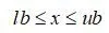
- lb = lower bound elements.
- up = upper bound elements.
- nonlcon = Nonlinear constrains.
- options = Output of optimoptions. (option = optimoption(‘SolverName’,’ Name’,’Value’)).
Explanation of Code:
The given function is defined based on the given expressions. The code for the given function is converted to a function so that the code can be used for the main solution. While defining the expression for the result function is entire equation is multiplied by the negative one so that the maxima can be found by calculating the minima of the function. This step is conducted because the genetic algorithm function in Matlab only gives minima of a function.
%Defining Staligmate function for GA studies.
function [f_xy] = stalig(input_vec)
x = input_vec(1);
y = input_vec(2);
f_x1 = (sin(5.1*pi*x+0.5))^6;
f_y1 = (sin(5.1*pi*y+0.5))^6;
f_x2 = exp((-4*0.6931)*(x-0.0667)^2/0.64);
f_y2 = exp((-4*0.6931)*(y-0.0667)^2/0.64);
f_xy = -f_x1*f_y1*f_x2*f_y2; %Output is multiplied with -1 so that maxima can be alter to minima
end
Code for the main solution:
Start with clearing all the variables, and the command workspace and closing all the plots that are still running.
clear all
close all
clc
Defining the input variables for the functions using linspace command to produce an array for inputs.
x = linspace(0, 0.6, 150);
y = linspace(0, 0.6, 150);
The input variable of x and y is tern to a 2D array by meshgrid command.
%Defining Mesh Grid for 2D array
[xx, yy] = meshgrid(x, y);
Calling defined function to record the output for the given input variables using a double for loop.
%staligmate call for output data collection of function
for i = 1:length(xx)
for j = 1:length(yy)
input_vec(1)=xx(i,j);
input_vec(2) = yy(i,j);
f(i,j) = stalig(input_vec);
end
end
The total number of iterations is defined for conducting the study.
iteration = 70; %Number of iterations
Study-1
Using an inbuild genetic algorithm calculating the local minima of function and their corresponding coordinate points. During the study, the genetic algorithm is only defined using the function and the number of variables. All the optimum values of the output of the function are stored in the variable ‘f_op’(an array of 1X150) and all the optimum input variable corresponding to the GA is stored in the variable ‘result’(Which contains 2 elements in every loop, the elements are x and y coordinate system corresponds to the output ‘f_op’).
%GA Study-1, Unbounded ga(fun,nvars)
for k = 1:iteration
[input f_op(k)] = ga(@stalig,2);
x_op(k) = input(1);
y_op(k) = input(2);
end
The results are displayed using the display command. The disp or display command is used to display the optimum values after the studies.
%Result
maxima = -stalig(input);
disp(['Maxima of function (f) = ',num2str(maxima)]);
disp(['X-coordinate = ',num2str(input(1))]);
disp(['y-coordinate = ',num2str(input(2))]);
The graph between the input x, y, and the output f is plotted using surfc command. The subplot command is used for showing for than one graph on a single figure. Colorbar command is used to map the color on the surface graph. Shading interp command is used to remove the line shading. A second plot is plotted on the same graph using plot3 and hold on commands to show the optimum values after the studies. The second graph or the subplot is plotted for the maxima vs iteration studies. The graph is decorated by using the xlabel, ylabel, tiltle, and grid on commands which label the x and y-axis, title the graph and turn to show the grid lines.
%Plot-1
figure(1);
subplot(2,1,1);
surfc(x, y, -f); %-f to reverse the output, so that the maximum can be visualised
colorbar;
shading interp;
hold on;
plot3(x_op, y_op, -f_op, 'Marker','*','MarkerSize',5,'color',[0.7 0.1 0.4]);
xlabel('x-coordinate[x]'); ylabel('y-coordinate[y]'); zlabel('output[f]');
hold off;
subplot(2,1,2);
plot(-f_op);
xlabel('Itration'); ylabel('Maxima')
grid on;
\\Analysis\\
The result was not good since the algorithm has no boundary it scans a wider area. Thus, the result becomes unsatisfactory.
Study-2
Here the same process is repeated with in a bounded region. The lower bound is x=0 and y=0 and the upper bound is x=0.6 and y=0.6.
%GA Study-2, bounded; ga(fun,nvars,A,b,Aeq,beq,lb,ub)
%lower bound x=0 y=0; upper bound x=0.6 y=0.6
for k = 1:iteration
[input, f_op(k)] = ga(@stalig,2,[],[],[],[],[0,0],[0.6,0.6]);
x_op(k) = input(1);
y_op(k) = input(2);
end
The results are displayed using the display command. The disp or display command is used to display the optimum values after the studies.
%Result
maxima = -stalig(input);
disp(['Maxima of function (f) = ',num2str(maxima)]);
disp(['X-coordinate = ',num2str(input(1))]);
disp(['y-coordinate = ',num2str(input(2))]);
The graph is plotted between the output and the corresponding input coordinates just like in study-1.
%plot-2
figure(2);
subplot(2,1,1);
surfc(x, y, -f); %-f to reverse the output, so that the maximum can be visualised
colorbar;
shading interp;
hold on;
plot3(x_op, y_op, -f_op, 'Marker','*','MarkerSize',2,'color',[0.7 0.1 0.4]);
xlabel('x-coordinate[x]'); ylabel('y-coordinate[y]'); zlabel('output[f]');
hold off;
subplot(2,1,2);
plot(-f_op);
xlabel('Itration'); ylabel('Maxima')
grid on;
\\Analysis\\
The result was much better but still, the population was not converged completely into a single region.
Study-3
Here in addition to the lower and upper bound the initial population is increased drastically.
%GA Study-3, ga(fun,nvars,A,b,Aeq,beq,lb,ub,nonlcon,options)
%lower bound x=0 y=0; upper bound x=0.6 y=0.6
%initial population rise to 300
options = optimoptions('ga','PopulationSize',300);
for k = 1:iteration
[input, f_op(k)] = ga(@stalig,2,[],[],[],[],[0,0],[0.6,0.6],[],options);
x_op(k) = input(1);
y_op(k) = input(2);
end
The results are displayed using the display command. The disp or display command is used to display the optimum values after the studies.
%Result
maxima = -stalig(input);
disp(['Maxima of function (f) = ',num2str(maxima)]);
disp(['X-coordinate = ',num2str(input(1))]);
disp(['y-coordinate = ',num2str(input(2))]);
The graph is plotted between the output and the corresponding input coordinates just like in study-1 and 2.
%plot-3
figure(3);
subplot(2,1,1);
surfc(x, y, -f); %-f to reverse the output, so that the maximum can be visualised
colorbar;
shading interp;
hold on;
plot3(x_op, y_op, -f_op, 'Marker','*','MarkerSize',2,'color',[0.7 0.1 0.4]);
xlabel('x-coordinate[x]'); ylabel('y-coordinate[y]'); zlabel('output[f]');
hold off;
subplot(2,1,2);
plot(-f_op,'linewidth',2);
xlabel('Itration'); ylabel('Maxima')
axis([0 70 0.99 1])
grid on;
\\Analysis\\
The sample space was converted to a single region and the result is very much satisfactory.
Error:
Error-1
Expression or statement is incomplete or incorrect.
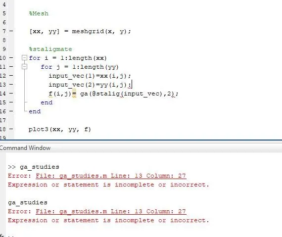
Solution: The statement was ended with a column instead of semi column. The column is substituted with a semi-column.
Error-2
Incorrect plot. The function plot got inverted.
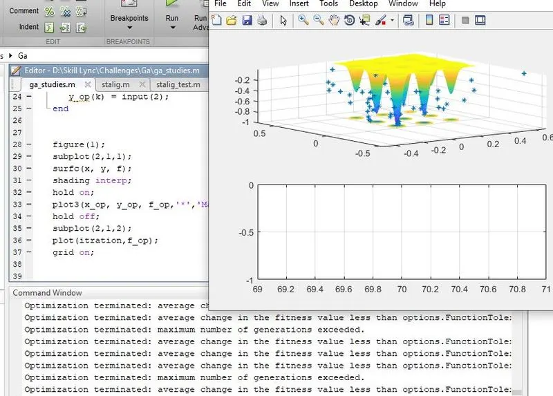
Solution: The function was inverted while defining the function, so have to be inverted back again by multiplying the output with the negative one while plotting.
Error-3
‘Sample_size’ was not an option for GA.
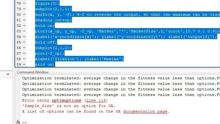
Solution: To increase the initial sample size the option inside the GA is population. So substituting sample_size with population.
Error-4
Incorrect size of InitialPopulationMatrix.
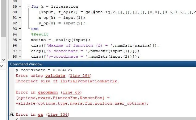
Solution: To increase the initial sample size the option inside the GA is PopulationSize. So substituting population with PopulationSize.
Reference:
https://in.mathworks.com/matlabcentral/answers/52240-how-to-find-max-fuction-with-genetic-algorithm
https://in.mathworks.com/help/gads/ga.html#d123e48598
https://en.wikipedia.org/wiki/Chromosome_(genetic_algorithm)