Week 3 - Solving second order ODEs
Code For The ODE Function.
function [dtheta_dt] = ode_func(t,theta,b,g,l,m)
theta1 = theta(1);
theta2 = theta(2);
dtheta1_dt = theta2;
dtheta2_dt = -(b/m)*theta2 - (g/l)*sin(theta1);

dtheta_dt = [dtheta1_dt; dtheta2_dt];
end
Code For The Solutopn And Animation.
%Pedulum Animation

%Input
g = 9.81; %m^2/s
l = 1; %m
b = 0.5; %damping coefficient
m = 1; %kg

% initial condition
theta_0 = [0;3];
%time positioning
t_span = linspace(0,20,500);

%solution for ODE
[t, results] = ode45(@(t, theta) ode_func(t, theta, b, g, l, m), t_span, theta_0);

%plot, time vs displacement and time vs angular velocity
figure(1);
plot(t, results(:,1),'color','b');
hold on;
plot(t, results(:,2),'color','r');
xlabel('Time(s)');
legend('Position','Angular Velocity');
grid on;
hold off;

%Animation
ct = 1;
for i = 1:length(t)
    omega = results(i,1);
    x0 = 0;
    y0 = 0;
    x1 = l*sin(omega);
    y1 = -l*cos(omega);

    figure(2);
    plot([x0 x1], [y0 y1], 'linewidth',3,'color','b');
    hold on;
    plot([-0.5 0.5], [0 0], 'linewidth',6,'color','g');
    plot(x0,y0,'Marker','o','MarkerFaceColor',[0 0 0], 'MarkerSize',3,'color',[0 0 0]);
    plot(x1,y1,'Marker','o','MarkerFaceColor','r', 'MarkerSize',12,'MarkerEdgeColor',[0 0 0]);
    axis([-2 2 -2 2]);
    grid on;
    title('Damping of Pendulum');
    xlabel('X-axis','color',[0 0 0]); ylabel('Y-axis','color',[0 0 0]);
    hold off;

    %Movie Making
    M(ct) = getframe(gcf);
    ct = ct+1;
end
movie(M);
videofile = VideoWriter('Damped Pendulum.avi', 'Uncompressed AVI');
videofile.FrameRate = 50;
open(videofile);
writeVideo(videofile, M);
close(videofile);
Explanation:
Code for the ODE function.
The ‘function’ and ‘end’ commands are used to turn the entire code into a function so that the function can be called while solving other problems.
The function is defined in terms of ‘t, theta, b, g, a’ and ‘l’. These variables are defined on the main solution. The calling out name of the function is ‘ode_func’
function [dtheta_dt] = ode_func(t,theta,b,g,l,m)
‘theta’ is a column matrix of two rows. The first element in the matrix is assigned to ‘theta1’ and the second element is assigned to ‘theta2’.
theta1 = theta(1);
theta2 = theta(2);
The given ODE is cut down to simple first-order ODEs. And the solution of both the ODEs are defined in terms of ‘dtheta1_dt’ and ‘dtheta2_dt’.
dtheta1_dt = theta2;
dtheta2_dt = -(b/m)*theta2 - (g/l)*sin(theta1);
The results of the function are defined in terms of a column matrix.
dtheta_dt = [dtheta1_dt; dtheta2_dt];
end
Code For Main Solution.
The given values are assigned to proper variables and defined.
%Pendulum Animation
%Input
g = 9.81; %m^2/s
l = 1; %m
b = 0.5; %damping coefficient
m = 1; %kg
The initial condition is defined in ‘theta_0’. Here the angular acceleration is 3rad/sec at 0 seconds. The variable ‘theta_0’ is defined in the column matrix because the solution of ODE is in the column matrix. The given time limit is from zero to 20 seconds, here 500 elements are selected from the given limit using ‘linspace’ command.
% initial condition
theta_0 = [0;3];
%time positioning
t_span = linspace(0,20,500);
The solution of the given ODE is calculated by the inbuild ‘ode45’ function. The earlier defined ‘ode_func’ is called inside the inbuild ‘ode45’ function. Here the ‘result’ contains two column matrixes. The first one is column contains displacement and the second column contains angular velocity.
%solution for ODE
[t, results] = ode45(@(t, theta) ode_func(t, theta, b, g, l, m), t_span, theta_0);
‘figure(1)’ command is used for defining the first figure since there are two figures in complete solution. The ‘plot’ command is used to plot between time(‘t’) and the angular displacement (‘results(:,1)’), the angular displacement is defined in the first column of ‘results’ matrix represents angular displacements in every time ‘t’. The ‘hold on’ command is used to plot multiple plots in a single figure.
%plot, time vs displacement and time vs angular velocity
figure(1);
plot(t, results(:,1),'color','b');
hold on;
The plot between time ‘t’ and angular velocity ‘results(:,2)’ is plotted using the command ‘plot’. The X-axis and Y-axis are titled using ‘xlabel’ and ‘ylabel’ respectively. ‘legend’ command is used to create disruptive labels in the figure(1) since it contains two plots. The grid is turned on for a better understanding of the graph. And the ‘hold off’ command is used to resent the ‘hold on’ command.
plot(t, results(:,2),'color','r');
xlabel('Time(s)');
legend('Position','Angular Velocity');
grid on;
hold off;
For making the animation the pendulum has to be defined. The animation is based on the position of the horizontal and vertical axis. The fixed point of the pendulum is defined with variables ‘x0’ and ‘y0’, and the endpoint of the pendulum is defined with variables ‘x1’ and ‘y1’ which change the position and speed with respect to the time period.
%Animation
ct = 1;
for i = 1:length(t)
omega = results(i,1);
x0 = 0;
y0 = 0;
x1 = l*sin(omega);
y1 = -l*cos(omega);
figure number two is defined using ‘figure(2)’ command. ‘plot’ command is used to plot the fixed-line and pendulum rod. The fixed-line is assumed to be a rod connecting the coordinate points (-0.5,0) and (0.5,0). The thickness for the fixed-line and the pendulum rode are given separately using the ‘linewidth’ command. And separate colors are assigned to each rod using ‘color’ command, for a better understanding of the plot.
figure(2);
plot([x0 x1], [y0 y1], 'linewidth',3,'color','b');
hold on;
plot([-0.5 0.5], [0 0], 'linewidth',6,'color','g');
The fixed end of the pendulum rod is marked with ‘O’ of marker width 3, and the oscillating end is also marked with ’O’ and a marker width 12. Each marker is colored differently using ‘color’ or ‘MarkerFaceColor’ command. Grind is turned on and the axis is labeled with titles for a better understanding of the plot. ‘hold on’ command is used to hold multiple plots on a single figure.
plot(x0,y0,'Marker','o','MarkerFaceColor',[0 0 0], 'MarkerSize',3,'color',[0 0 0]);
plot(x1,y1,'Marker','o','MarkerFaceColor','r', 'MarkerSize',12,'MarkerEdgeColor',[0 0 0]);
axis([-2 2 -2 2]);
grid on;
title('Damping of Pendulum');
xlabel('X-axis','color',[0 0 0]); ylabel('Y-axis','color',[0 0 0]);
hold off;
The animation is then converted into a movie. ‘getframe(gcf)’ is used to capture each current figure and stored inside the array M. A video file is created by ‘VideoWriter’ command, also the file is named (‘Damped Pendulum.avi’) while creating the file. The frame refresh rate is assigned by using ‘videofile.FrameRate’ command. The created video file is opened and the captured figures in array ‘M’ are written to the video file with help of ‘writeVideo’ command. After writing the video, the file is closed.
%Movie Making
M(ct) = getframe(gcf);
ct = ct+1;
end
movie(M);
videofile = VideoWriter('Damped Pendulum.avi', 'Uncompressed AVI');
videofile.FrameRate = 50;
open(videofile);
writeVideo(videofile, M);
close(videofile);
Result:
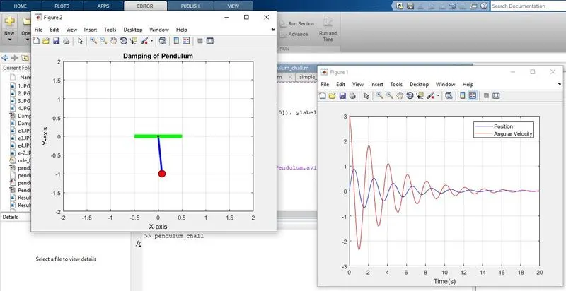
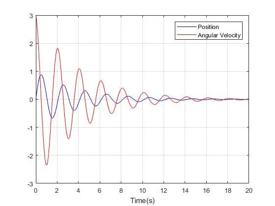
Errors:
Error-1
Undefined function or variable error.
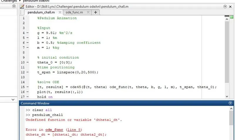
Solution: While defining ‘dtheta_dt’ there was a spelling mistake. ‘dtheta_dt’ is defined properly.
Error-2
Unbalanced or unexpected parenthesis.
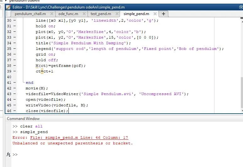
Solution: While closing the video file there was a dot inside the parenthesis which is removed to remove the error.
Error-3
Improper command definition.
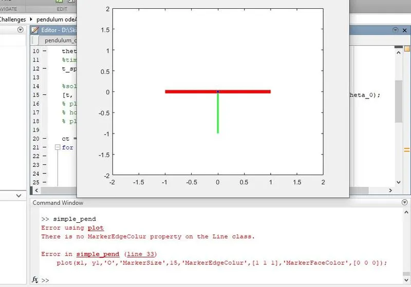
Solution: The ‘MarkerEdgeColur’ is replaced by ‘MarkerEdgeColor’ to remove the error.
Error-4
Mistake while defining the ‘legend’ command.
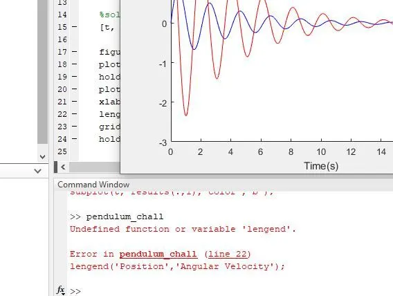
Solution: The command ‘lengend’ is substituted with ‘legend’ to remove the error.
Error-5
Wrong animation definition.
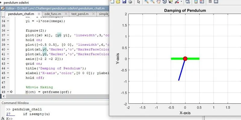
Solution:
The plot definition for the bob was wrongly defined. The coordinate points ‘x0’, and ‘y0’ is replaced with ‘x1’ and ‘x2’.
Error-6
Error in the animation video.
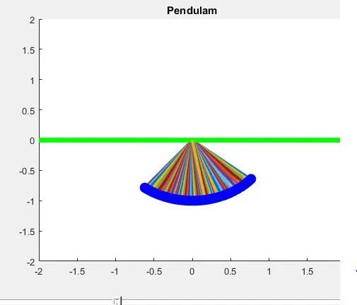
Solution: ’hold on’ command was defined early. The command is defined after the first plot definition.
Video link: https://youtu.be/MeysfrJlzMI