Week 4.1 - Genetic Algorithm

AIM: Write a code in MATLAB to optimize the stalagmite function.

OBJECTIVE:

• Write a code in MATLAB to optimize the stalagmite function and find the global maxima of the function.
• Clearly explain the concept of genetic algorithm and also explain the syntax for ga in MATLAB.
• Plot graphs for all 3 studies and for F maximum vs no. of iterations.

THEORY:

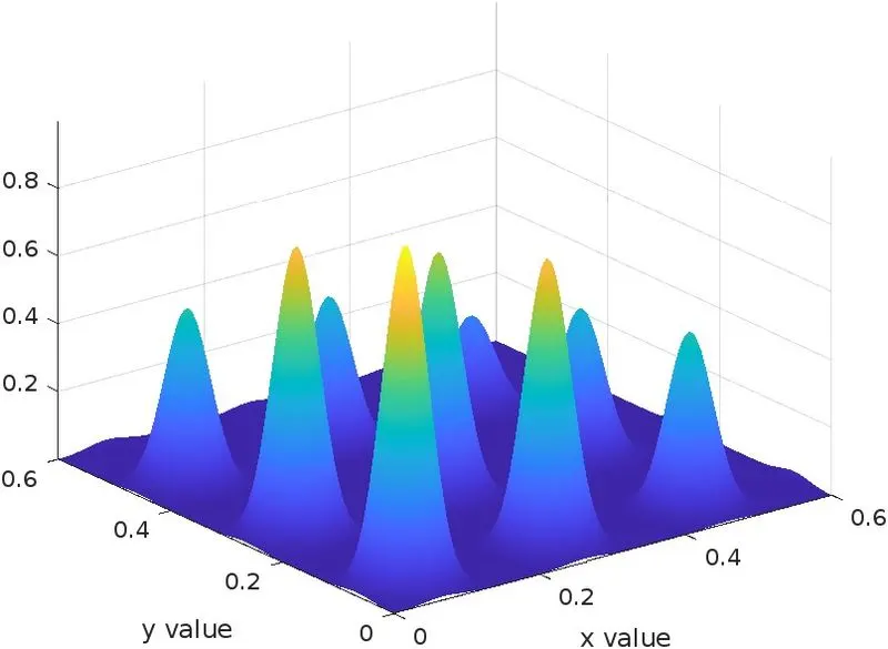
Stalagmite is a type of rock formation that rises from the floor of a cave due to the accumulation of material deposited on the floor from ceiling drippings. Similarly, the stalagmite function generally refers to the function with which we are generating values over a stalagmite kind of surface for finding out the local and global maxima and minima of that particularly given function.

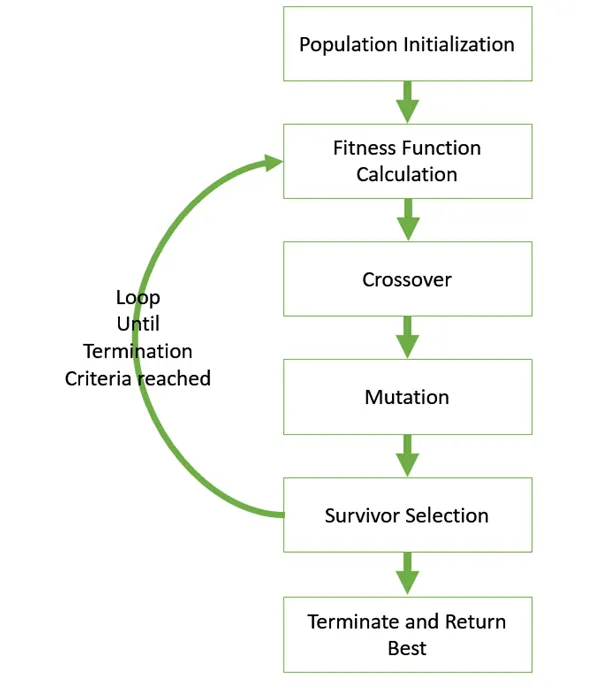
A Genetic Algorithm is an optimization technique used to solve nonlinear optimization problems. It uses the concept from evolutionary biology. It is frequently used to find optimal or near-optimal solutions to difficult problems which otherwise would take a lifetime to solve. It consists of three genetic operators - selection operator, crossover operator, and mutation operator which enables us to find an optimal solution by 'ga'.

Basic Structure of GA

Syntax that we use in our problem:

1. x = ga(fun,nvars)

2. x = ga(fun,nvars,A,b,Aeq,beq,lb,ub)

3. x = ga(fun,nvars,A,b,Aeq,beq,lb,ub,nonlcon,options)

where,

fun = the objective function

nvars = number of design variables of objective function.

A,B,Aeq,beq are terms of linear inequalities A*x ≤ b and Aeq*x = beq

'lb' lower and 'ub' upper bounds on the design variables

nonlcon = Nonlinear Constraints (eg. x^2 + y^3>=2)

options = optimization parameters replaced by values in options

But in this case we are not considering A,B,Aeq,beq,nonlcon parameters in the 'ga' syntax so we replace them with '[]'.

In syntax 1, finds a local unconstrained minimum, x, to the objective function, fun. nvars is the dimension (number of design variables) of fun.

In syntax 2, defines a set of lower and upper bounds on the design variables, x, so that a solution is found in the range lb ≤ x ≤ ub.

In syntax 3, minimizes with the default optimization parameters replaced by values in options.

Stopping Criteria of ga:

1. Generations: when the generation reaches this predefined value, it stops and provides the best solution in the last generation.

2. Time Limit: algorithm stops when it reaches a predefined time limit.

3. Fitness limit: algorithm stops when the value of the fitness function for the best point in the current population is less than or equal to the fitness limit.

We do 3 studies on 'ga' to identify how the ga function value can improve or give a more consistent value for function minimum using extra criteria for ga like lower bound, upper bound, options, etc.

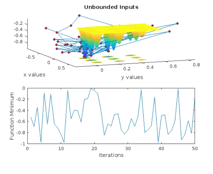
Study 1 - by running this we can how ga predict the value for function minimum.

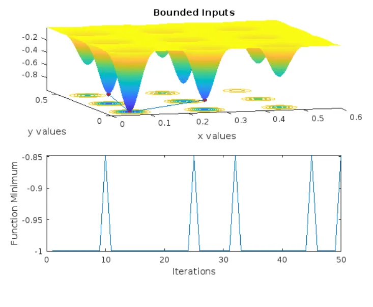
Study 2 - in addition to study 1, we add boundary conditions to it.

Study 3 - in addition to study 2 we increase the iteration time for ga.

EQUATION:

f_1,x=[sin(5.1πx+0.5)]⁶
f_1,y=[sin(5.1πy+0.5)]⁶
f_2,x=exp[-4*ln(2)(x-0.0667)²/0.64]
f_2,y=exp[-4*ln(2)((y-0.0667)²/0.64)]

To find global maxima,

f(x,y) = f_1,x*f_1,y*f_2,x*f_2,y

To find global minima,

f(x,y) = -( f_1,x*f_1,y*f_2,x*f_2,y)

PROGRAM FOR MATLAB:

To find the global minima

clear all                           %clear the workspace if there any previus data exist.
close all                           %close all figures and plots
clc                                 %clear the command window if there any previus data exist.

% A program for finding global maxima
%defining our search space
x = linspace(0,0.6,150);
y = linspace(0,0.6,150);

%creating a 2dimensional mesh
[xx, yy] = meshgrid(x,y);

for i = 1 : length(xx)  
    for j = 1 : length(yy)
        input_vector(1) = xx(i,j);  
        input_vector(2) = yy(i,j);
        f(i,j) = stalagmite(input_vector);
        
    end
end
 surfc(xx,yy,f) %creates a three-dimensional surface plot with a contour plot underneath
 xlabel('x value')
 ylabel('y value')
 shading interp %the color in each line segment and face by interpolating the colormap index

 [inputs,fval] = ga(@stalagmite,2)  %ga function used to find a local unconstarined minima with 2 variables x and y.

 function [f] = stalagmite(input_vector) %named the function a s stalagmite with input variable as 'input_vector'.

X = input_vector(1);    %assign input_vector(1) as 'X'
Y = input_vector(2);    %assign input_vector(2) as 'Y'

%equation1
term1 = 5.1*pi*X + 0.5;
f1_X = (sin(term1))^6;

%equation2
term2 = 5.1*pi*Y + 0.5;
f1_Y = (sin(term2))^6;

%equation3
term3 = (-4*log(2))/0.64;
term4 = (X-0.0667)^2;
f2_X = exp(term3*term4);

%equation4
term5 = (Y-0.0667)^2;
f2_Y = exp(term3*term5);

[f] = f1_X*f1_Y*f2_X*f2_Y;  %relation connecting all equations.
end

To find the global maxima and three studies for finding optimized 'ga' value.

clear all                           %clear the workspace if there any previus data exist.
close all                           %close all figures and plots
clc                                 %clear the command window if there any previus data exist.

%defining our search space
x = linspace(0,0.6,150);    
y = linspace(0,0.6,150);

%creating a 2dimensional mesh
[xx, yy] = meshgrid(x,y);

for i = 1 : length(xx)  %for loop for defining the row number
    for j = 1 : length(yy)  %for loop for defining the column numer
        input_vector(1) = xx(i,j);  %assign the 'xx' (i,j) value to input_vector(1)
        input_vector(2) = yy(i,j);  %assign the 'yy' (i,j) value to input_vector2)
        f(i,j) = stalagmite(input_vector);  %calling the function
        
    end
end

num_cases = 50; %running "ga' for 50 times

tic %for recording time, and time start to count now
%Study 1 -Statistical Behaviour
for i = 1:num_cases %this loop give running criteria for ga function
    [inputs,fopt(i)] = ga(@stalagmite,2);   %calling ga with objective function as stalagmite and design variables 2.
    xopt(i) = inputs(1);    %assign input(1) as xopt
    yopt(i) = inputs(2);    %assign input(2) as yopt
end
study1_time = toc   %time recording till now


figure(1)   %creates a figure
subplot(2,1,1)  %help us  to occupy multiple plots within a single figure.This divides the current figure into an 
                % 2 by 1 grid and creates an axes 1.
hold on %retains plots in the current axes so that new plots added to the axes do not delete existing plots
surfc(xx,yy,f)  %creates a three-dimensional surface plot with a contour plot underneath
shading interp  %the color in each line segment and face by interpolating the colormap index
plot3(xopt,yopt,fopt,'marker','o','markersize',5,'MarkerFaceColor','r') %creates a 3d plot with points marker as red dots.
xlabel('x values')  %named x axis
ylabel('y values')  %named y axis
title('Unbounded Inputs')   %named title
subplot(2,1,2)  %help us  to occupy multiple plots within a single figure.This divides the current figure into an 2 by 1 grid and creates axes by 2.
plot(fopt)  %creates a new plot 
xlabel('Iterations')    %named x axis
ylabel('Function Minimum')  %named y axis


tic %for recording time, and time start to count now
%Study 2 -Statistical Behaviour with upper and lower bounds
for i = 1:num_cases %this loop give running criteria for ga function
    [inputs,fopt(i)] = ga(@stalagmite,2,[],[],[],[],[0;0],[0.4;0.45]);  %ga calculation is limited to lower and upper bounds 
                                                                        % that is 0 to 0.4 in x axis and 0 to 0.45 in y axis 
    xopt(i) = inputs(1);
    yopt(i) = inputs(2);
end
study2_time = toc   %time recording till now


figure(2)
subplot(2,1,1)
hold on
surfc(xx,yy,f)
shading interp
plot3(xopt,yopt,fopt,'marker','o','markersize',5,'MarkerFaceColor','r')
xlabel('x values')
ylabel('y values')
title('Bounded Inputs')
subplot(2,1,2)
plot(fopt)
xlabel('Iterations')
ylabel('Function Minimum')



%Study 3 -Increasing GA Iterations
options = optimoptions('ga');   %taking ga to optimization
options = optimoptions(options,'PopulationSize',170);   %increase the populationsize to 170. So ga running 170 times.

tic %for recording time, and time start to count now
for i = 1:num_cases %this loop give running criteria for ga function
    [inputs,fopt(i)] = ga(@stalagmite,2,[],[],[],[],[0;0],[0.4;0.45],[],[],options);    %new changed population size is applied to the ga function.
    xopt(i) = inputs(1);
    yopt(i) = inputs(2);
end
study3_time = toc   %time recording till now


figure(3)
subplot(2,1,1)
hold on
surfc(xx,yy,f)
shading interp
plot3(xopt,yopt,fopt,'marker','o','markersize',5,'MarkerFaceColor','r')
xlabel('x values')
ylabel('y values')
title('Bounded Inputs')
subplot(2,1,2)
plot(fopt)
xlabel('Iterations')
ylabel('Function Minimum')

 function [f] = stalagmite(input_vector) %named the function a s stalagmite with input variable as 'input_vector'.

X = input_vector(1);    %assign input_vector(1) as 'X'
Y = input_vector(2);    %assign input_vector(2) as 'Y'

%equation1
term1 = 5.1*pi*X + 0.5;
f1_X = (sin(term1))^6;

%equation2
term2 = 5.1*pi*Y + 0.5;
f1_Y = (sin(term2))^6;

%equation3
term3 = (-4*log(2))/0.64;
term4 = (X-0.0667)^2;
f2_X = exp(term3*term4);

%equation4
term5 = (Y-0.0667)^2;
f2_Y = exp(term3*term5);

[f] = -1*f1_X*f1_Y*f2_X*f2_Y;  %relation connecting all equations. (-1) use to convert the maxima problem to minima.
end

OUTPUT PLOTS:

1. Global Maxima

2. Study 1 -Statistical Behaviour

3. Study 2 -Statistical Behaviour with upper and lower bounds

4. Study 3 -Increasing GA Iterations

RESULTS:

• We did three iterations in 'ga' ie, studies 1,2, & 3. At study 1, the ga output points are randomly oriented without any limit, these can be seen in study 1 output plot. And the function minimum value is kept varying.

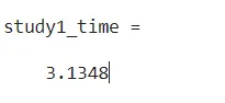
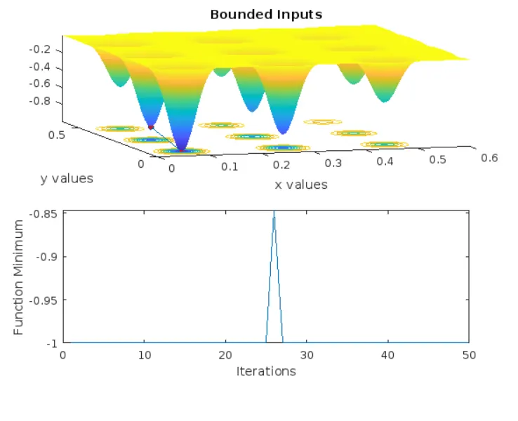
• At study 2 we give boundary conditions by using 'lb' and 'up' in ga function. So the ga output points are limited to the 3d stalagmite projection. This ga takes much more time to process than study 1 and the iteration graph is better.

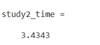
• At study 3 we give increase the iteration of ga from 50 to 170 in addition to the boundary, this iterates the function minimum value ie, other than one point it gives an optimal solution, this also takes more simulation time.

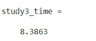
• So by giving boundary conditions and increasing population size we get a well-optimized value for the function. By giving more conditions we can modify the ga result that results in an optimal solution. We can also add linear conditions and non-linear conditions to the ga if we need.
• GA makes optimization a bit easier, and stalagmite visualization helps us to find the minimas and maximas.