Project 2 - Rankine cycle Simulator
AIM: Create a Rankine Cycle Simulator using OCTAVE/MATLAB.
OBJECTIVES:
- Calculate the state points of the Rankine Cycle based on user inputs using MATLAB.
- Plot the corresponding T-s and h-s plots for the given set of inputs.
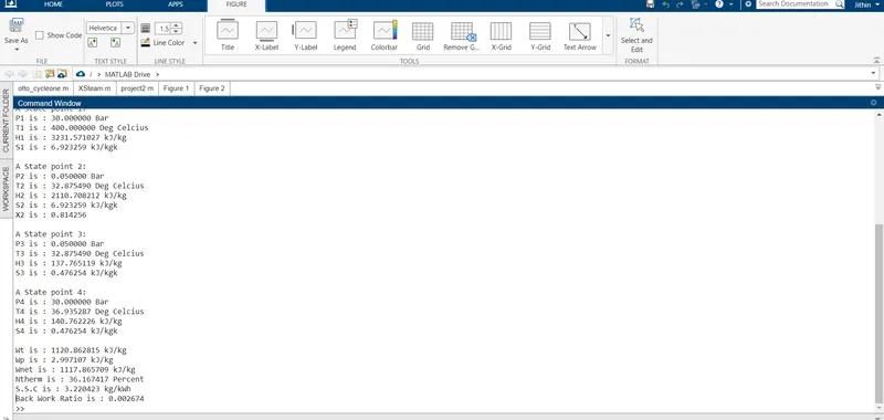
- Calculate net work output and back work ratio.
THEORY:
Rankine cycle is an idealized thermodynamic cycle of a constant pressure heat engine that converts part of heat into mechanical work. In this cycle, the heat is supplied externally to a closed loop, which usually uses water (in a liquid and vapor phase) as the working fluid.
Rankine cycle describes the performance of steam turbine systems, though the theoretical principle also applies to reciprocating engines such as steam locomotives.
Rankine Cycle - Processes
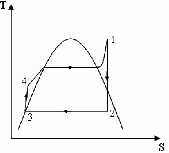
In an ideal Rankine cycle, the system executing the cycle undergoes a series of four processes: two isentropic (reversible adiabatic) processes alternated with two isobaric processes:
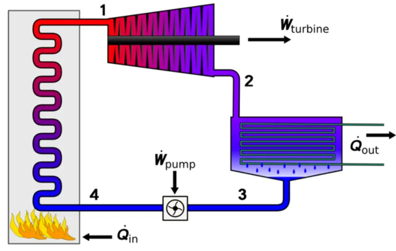
Components of Rankine Cycle:
- Turbine
- Condenser
- Pump
- Boiler
Processes:
- Process 1-2: Isentropic expansion in a turbine. The dry saturated vapour expands through the turbine resulting in the generation of power.
Wt = m(h1-h4)
- Process 2-3: Constant pressure heat rejection in a condenser. Wet vapour is condensed at a constant pressure to become a saturated liquid
Qout = m(h2-h3)
- Process 3-4: Isentropic compression in a pump. Here the working fluid is pumped from low to high pressure
Wp = m(h3-h4)
- Process 4-1: Constant pressure heat addition in the boiler. In this process, the high-pressure liquid is added to the boiler and is heated at constant pressure to become a dry saturated vapour.
Qin = m(h4-h1)
EQUATIONS USED:
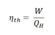
Thermal Efficiency of Rankine Cycle
In general, the thermal efficiency, ηth, of any heat engine is defined as the ratio of the work it does, W, to the heat input at the high temperature, QH.
Dryness fraction
General equation,
x = ms / ms + mw
where,
ms = Mass of Dry Steam
mw = Weight of Water Particles in Suspension in Steam.
But we use,
Required Inputs:
Turbine Inlet temperature = 400° C
Turbine Inlet Pressure = 30 bars
Turbine Outlet Pressure = 0.05 bars = Condenser Inlet Pressure
clear all                           %clear the workspace if there any previus data exist.
close all                           %close all figures and plots
clc                                 %clear the command window if there any previus data exist.

% T     Temperature (deg C)
% p	    Pressure    (bar)
% h	    Enthalpy    (kJ/kg)
% v	    Specific volume (m3/kg)
% s	    Specific entropy
% Cp	Specific isobaric heat capacity
% Cv	Specific isochoric heat capacity
%hV_p	Saturated vapour enthalpy
%hL_p	Saturated liquid enthalpy
%h_pT	Entalpy as a function of pressure and temperature.
%h_ps	Entalpy as a function of pressure and entropy.
%sV_p	Saturated vapour entropy
%sL_p	Saturated liquid entropy
%s_pT	Specific entropy as a function of pressure and temperature
%Cp_ps	Specific isobaric heat capacity as a function of pressure and entropy.
%Cv_ps	Specific isochoric heat capacity as a function of pressure and entropy.


% A program to create a rankine simulator
disp('RANKINE CYCLE SIMULATOR')     %disp command shows the character in the command box.
disp(' ')
disp('1-2 is Isentropic Expansion in the Turbine')
disp('2-3 is Const Pressure Heat Rejection by the Condenser')
disp('3-4 is Isentropic Compression in the pump')
disp('4-1 Const Pressure Heat Addition by the Boiler')
disp(' ')
%User Input
p1 = input('Enter the Pressure at the Turbine Inlet (in bar): ');   %input command request user for input
T1 = input('Enter the Temperature at the Turbine Inlet (in Degree Celcius): ');
p2 = input('Enter the Pressure at the Condenser (in bar): ');
3. Taking values for each from XSteam Library
By using XSteam library each value is calculated. hV_p, hL_p, h_pT, h_ps, sV_p, sL_p, s_pT, Cp_ps, Cv_ps etc. are used to pick corresponding values from XSteam library.
Code:
%State point 1 (turbine inlet/boiler outlet)
s1 = XSteam('s_pT',p1,T1);      %Specific entropy at state point 1.
h1  = XSteam('h_pT',p1,T1);     %Specific enthalphy at state point 1.

%State point 3 on the staturation line
%State point 3 (pump inlet/condenser outlet)
p3 = p2;         %because 2-3 is an isobaric process
sf3 = XSteam('sL_p',p3);    %Specific entropy in liquid at p3 pressure extracted from XSteam library and assign the value to sf3.
hf3  =XSteam('hL_p',p3);    %Specific enthalphy in liquid at p3 pressure extracted from XSteam library and assign the value to hf3.
vf3 = XSteam('vL_p',p3);    %Specific volume in liquid at p3 pressure extracted from XSteam library and assign the value to vf3.
s3 = sf3;                   %because 3 is on saturation curve
h3 = hf3;                   %because 3 is on saturation curve
T3 = XSteam('Tsat_p',p3);   %T3 is saturation temperature at p3 pressure extracted from XSteam library using 'Tsat_p'


%State point 2 (turbine outlet/condenser inlet)
s2 = s1;                    %1-2 is an Isentropic process
sf2 = XSteam('sL_p',p2);    %Specific entropy in liquid at p2 pressure extracted from XSteam library and assign the value to sf2.
sg2 = XSteam('sV_p',p2);    %Specific entropy in vapour at p2 pressure extracted from XSteam library and assign the value to sg2.
sfg2 = (sg2-sf2);           %sfg is  difference between sg and sf.
hf2 = XSteam('hL_p',p2);    %Specific enthalphy in liquid at p2 pressure extracted from XSteam library and assign the value to hf2.
hg2 = XSteam('hV_p',p2);    %Specific enthalphy in vapour at p2 pressure extracted from XSteam library and assign the value to hg2.
hfg2 = (hg2-hf2);           %hfg is  difference between hg and hf.
x2 = ((s2-sf2)/sfg2);       %dryness fraction
h2 = hf2 + (x2*hfg2);       %Specific enthalphy at state point 2
T2 = T3;  %Temperature at state point 2. T2 and T3 are inside saturation curve.


%State point 4 (pump outlet/boiler inlet)
p4 = p1;                    %because 4-1 is an isobaric process
s4 = s3;                    %because 3-4 is an isoentropic process
h4 = XSteam('h_ps',p4,s4);  %Specific enthalphy at p4 pressure and s4 entropy extracted from XSteam library and assign the value to h4.
Cp4 = XSteam('Cp_ps',p4,s4);    %Specific isobaric heat capacity as a function of pressure 'p4' and entropy 's4' extracted from XSteam library and assign to Cp4.
Cv4 = XSteam('Cv_ps',p4,s4);    %Specific isochoric heat capacity as a function of pressure 'p4' and entropy 's4'extracted from XSteam library and assign to Cv4.
gamma = Cp4/Cv4;    %gamma is the ratio b/w Cp/Cv
r = (gamma-1)/gamma;
T4 = T3*(p4/p3)^r;  %isentropic relation


%State point 5 & 6 (points on saturation curve)
T5 = XSteam('Tsat_p',p1);   %Saturation temperature in p1 pressure extracted from XSteam library and assign the value to T5.
T6 = T5;        %beacuse 5 and 6 are on saturation curve then temperature becomes same
s5 = XSteam('sL_p',p1); %Specific entropy in liquid at p1 pressure extracted from XSteam library and assign the value to s5.
s6 = XSteam('sV_p',p1); %Specific entropy in vapour at p1 pressure extracted from XSteam library and assign the value to s6.
h5 = XSteam('hL_p',p1); %Specific enthalphy in liquid at p1 pressure extracted from XSteam library and assign the value to h5.
h6 = XSteam('hV_p',p1); %Specific enthalphy in vapor at p1 pressure extracted from XSteam library and assign the value to h6.
4. Plotting T-s Diagram
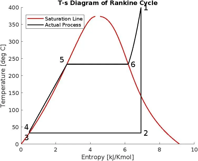
First we create values for plotting saturation curve, for that first we create an array of value using linspace command and assign the value to 't'. Then, for loop is created that finds entropy in liquid and vapour phase corresponding to 't' array. Next,we create values for plotting temperature saturation line, for that we create array from T5 temperature to T1 temperature with 500 points and it is assign to 'n', then using for loop entropy is calculated using constant pressure and 'n' array.
Afterwards, we plots the curves using plot command and mark the corresponding points using text command, in addition we use 'VerticalAlignment', 'HorizontalAlignment' and 'fontsize' are used to set proper text properties. Legend command used to descriptive the labels.
Code:
%plotting T-s diagram
figure(1)   %figure 1 is created.
hold on     %retains plots in the current axes so that new plots added to the axes do not delete existing plots

%For loop for saturation Curve
t = linspace(0,400,500);    %temperature array is created with 500 points.
for i = 1:length(t)
    s_L(i) = XSteam('sL_T',t(i));
    s_V(i) = XSteam('sV_T',t(i));
end

%For loop for saturation temperature line at p1 pressure.
n = linspace(T5,T1,500);    %temperature array is created from T5 to T1 temperature with 500 points.
for j =1:length(n)
    s(j) = XSteam('s_pT',p1,n(j));
end


%line plotting
plot([s_L s_V],[t t],'-r','LineWidth',1.5)      %plot saturation curve
plot([s1,s2 s3 s4 s5 s6 s],[T1,T2 T3 T4 T5 T6 n],'-k','LineWidth',1.5)  %plot actual process

legend('Saturation Line','Actual Process') %descriptive the labels.

%marking points
text(s1,T1,' 1','fontsize',14)  %marking point 1
text(s2,T2,' 2','fontsize',14)  %marking point 2
text(s3,T3,' 3','VerticalAlignment','top','HorizontalAlignment','right','fontsize',14)   %marking point 3
text(s4,T4,'  4','VerticalAlignment','bottom','HorizontalAlignment','right','fontsize',14)    %marking point 4
text(s5,T5,'5 ','VerticalAlignment','bottom','HorizontalAlignment','right','fontsize',14)    %marking point 5
text(s6,T6,' 6','fontsize',14)  %marking point 6


%naming
xlabel('Entropy [kJ/Kmol]') %naming x-axis
ylabel('Temperature [deg C]')   %naming y-axis
title('T-s Diagram of Rankine Cycle')   %naming title
hold off    %stop retaining plots in the current axes
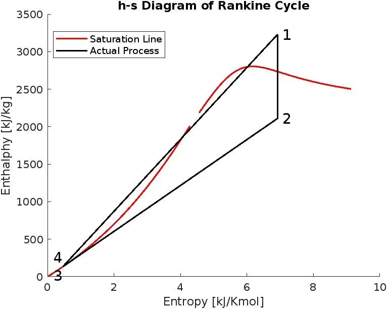
5. Plotting h-s Diagram
Similar to T-s plotting, only is in for loop values. In this for loop we find entropy and enthalphy corresponding to the temperature value array 'k'. Using that values h-s saturation curve is plotted using plot command. All other things are same as T-s diagram.
Code:
%plotting h-s diagram
figure(2)   %figure 2 is created
hold on     %retains plots in the current axes so that new plots added to the axes do not delete existing plots

%For loop for saturation Curve
k = linspace(0,400,500);    %temperature array is created with 500 points.
for l = 1:length(k)
    s_L(l) = XSteam('sL_T',k(l));
    s_V(l) = XSteam('sV_T',k(l));
    h_L(l) = XSteam('hL_T',k(l));
    h_V(l) = XSteam('hV_T',k(l));
end

%plotting lines
plot([s_L s_V],[h_L h_V],'-r','LineWidth',1.5)      %plot saturation curve
plot([s1 s2 s3 s4 s1],[h1 h2 h3 h4 h1],'-k','LineWidth',1.5)    %plot actual process

legend('Saturation Line','Actual Process')  %descriptive the labels.

%marking points
text(s1,h1,' 1','fontsize',14)   %marking point 1
text(s2,h2,' 2','fontsize',14)   %marking point 2
text(s3,h3,' 3','VerticalAlignment','top','HorizontalAlignment','right','fontsize',14)   %marking point 3
text(s4,h4,'   4','VerticalAlignment','bottom','HorizontalAlignment','right','fontsize',14) %marking point 4

%naming
xlabel('Entropy [kJ/Kmol]') %naming x-axis
ylabel('Enthalphy [kJ/kg]') %naming y-axis
title('h-s Diagram of Rankine Cycle')   %naming title
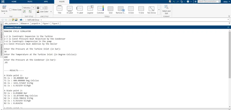
6. Display results
We use fprintf command for display the data as text. At proper position we add values that already found using '%f'.
Code:
%Details to be displayed
fprintf('\n\n-----RESULTS-----\n')
fprintf('\nA State point 1:\nP1 is : %f Bar\nT1 is : %f Deg Celcius\nH1 is : %f kJ/kg\nS1 is : %f kJ/kgk',p1,T1,h1,s1)    %write datas as text
fprintf('\n\nA State point 2:\nP2 is : %f Bar\nT2 is : %f Deg Celcius\nH2 is : %f kJ/kg\nS2 is : %f kJ/kgk\nX2 is : %f',p2,T2,h2,s2,x2)
fprintf('\n\nA State point 3:\nP3 is : %f Bar\nT3 is : %f Deg Celcius\nH3 is : %f kJ/kg\nS3 is : %f kJ/kgk',p3,T3,h3,s3)
fprintf('\n\nA State point 4:\nP4 is : %f Bar\nT4 is : %f Deg Celcius\nH4 is : %f kJ/kg\nS4 is : %f kJ/kgk\n\nWt is : %f kJ/kg\nWp is : %f kJ/kg\nWnet is : %f kJ/kg\nNtherm is : %f Percent\nS.S.C is : %f kg/kWh\n Back Work Ratio is : %f\n',p4,T4,h4,s4,Wt,Wp,Wnet,Ntherm,steam_rate,BWR)
clear all                           %clear the workspace if there any previus data exist.
close all                           %close all figures and plots
clc                                 %clear the command window if there any previus data exist.

% T     Temperature (deg C)
% p	    Pressure    (bar)
% h	    Enthalpy    (kJ/kg)
% v	    Specific volume (m3/kg)
% s	    Specific entropy
% Cp	Specific isobaric heat capacity
% Cv	Specific isochoric heat capacity
%hV_p	Saturated vapour enthalpy
%hL_p	Saturated liquid enthalpy
%h_pT	Entalpy as a function of pressure and temperature.
%h_ps	Entalpy as a function of pressure and entropy.
%sV_p	Saturated vapour entropy
%sL_p	Saturated liquid entropy
%s_pT	Specific entropy as a function of pressure and temperature
%Cp_ps	Specific isobaric heat capacity as a function of pressure and entropy.
%Cv_ps	Specific isochoric heat capacity as a function of pressure and entropy.


% A program to create a rankine simulator
disp('RANKINE CYCLE SIMULATOR')     %disp command shows the character in the command box.
disp(' ')
disp('1-2 is Isentropic Expansion in the Turbine')
disp('2-3 is Const Pressure Heat Rejection by the Condenser')
disp('3-4 is Isentropic Compression in the pump')
disp('4-1 Const Pressure Heat Addition by the Boiler')
disp(' ')

p1 = input('Enter the Pressure at the Turbine Inlet (in bar): ');   %input command request user for input
T1 = input('Enter the Temperature at the Turbine Inlet (in Degree Celcius): ');
p2 = input('Enter the Pressure at the Condenser (in bar): ');


%Considered state point 1 on the staturation line
%State point 1 (turbine inlet/boiler outlet)
s1 = XSteam('s_pT',p1,T1);      %Specific entropy at state point 1.
h1  = XSteam('h_pT',p1,T1);     %Specific enthalphy at state point 1.

%State point 2 (turbine outlet/condenser inlet)
s2 = s1;
sf2 = XSteam('sL_p',p2);    %Specific entropy in liquid at p2 pressure is extracted from XSteam library and assign the value to sf2.
sg2 = XSteam('sV_p',p2);    %Specific entropy in vapour at p2 pressure is extracted from XSteam library and assign the value to sg2.
sfg2 = (sg2-sf2);           %sfg is  difference between sg and sf.
hf2 = XSteam('hL_p',p2);    %Specific enthalphy in liquid at p2 pressure is extracted from XSteam library and assign the value to hf2.
hg2 = XSteam('hV_p',p2);    %Specific enthalphy in vapour at p2 pressure is extracted from XSteam library and assign the value to hg2.
hfg2 = (hg2-hf2);           %hfg is  difference between hg and hf.
x2 = ((s2-sf2)/sfg2);       %dryness fraction
h2 = hf2 + (x2*hfg2);       %Specific enthalphy at state point 2
T2 = XSteam('T_ph',p2,h2);  %Temperature at state point 2.


%State point 3 on the staturation line
%State point 3 (pump inlet/condenser outlet)
p3 = p2;         %because 2-3 is an isobaric process
sf3 = XSteam('sL_p',p3);    %Specific entropy in liquid at p3 pressure is extracted from XSteam library and assign the value to sf3.
hf3  =XSteam('hL_p',p3);    %Specific enthalphy in liquid at p3 pressure is extracted from XSteam library and assign the value to hf3.
vf3 = XSteam('vL_p',p3);    %Specific volume in liquid at p2 pressure is extracted from XSteam library and assign the value to hf2.
s3 = sf3;                   %because 3 is on saturation curve
h3 = hf3;                   %because 3 is on saturation curve
T3 = T2;                    %beacuse 2 and 3 are inside saturation curve then temperature becomes same

%State point 4 (pump outlet/boiler inlet)
p4 = p1;                    %because 4-1 is an isobaric process
s4 = s3;                    %because 3-4 is an isoentropic process
h4 = XSteam('h_ps',p4,s4);  %Specific enthalphy at p4 pressure and s4 entropy is extracted from XSteam library and assign the value to h4.
Cp4 = XSteam('Cp_ps',p4,s4);
Cv4 = XSteam('Cv_ps',p4,s4);
%gamma = Cp4/Cv4;
%r = (gamma-1)/gamma
T4 = XSteam('T_ps',p4,s4);  %Temperature at p4 pressure and s4 entropy is extracted from XSteam library and assign the value to T4.


%State point 5 & 6
T5 = XSteam('Tsat_p',p1);   %Saturation temperature in p1 pressure is extracted from XSteam library and assign the value to T5.
T6 = T5;        %beacuse 5 and 6 are on saturation curve then temperature becomes same
s5 = XSteam('sL_p',p1); %Specific entropy in liquid at p1 pressure is extracted from XSteam library and assign the value to s5.
s6 = XSteam('sV_p',p1); %Specific entropy in vapour at p1 pressure is extracted from XSteam library and assign the value to s6.
h5 = XSteam('hL_p',p1); %Specific enthalphy in liquid at p1 pressure is extracted from XSteam library and assign the value to h5.
h6 = XSteam('hV_p',p1); %Specific enthalphy in vapor at p1 pressure is extracted from XSteam library and assign the value to h6.


%Turbine work
Wt = h1-h2;

%Pump work
Wp = h4-h3;

%Net work ouput of the cycle
Wnet = Wt - Wp;

%Heat input
Qin = h1-h4;

%Heat output
Qout = h2-h3;

%Thermal Efficiency [%]
Ntherm = (Wnet/Qin)*100;

%Steam Rate
steam_rate = 3600/(Wt-Wp);


%plotting T-s diagram
figure(1)   %figure 1 is created.
hold on     %retains plots in the current axes so that new plots added to the axes do not delete existing plots

%For loop for saturation Curve
t = linspace(0,400,500);    %temperature array is created with 500 points.
for i = 1:length(t)
    s_L(i) = XSteam('sL_T',t(i));
    s_V(i) = XSteam('sV_T',t(i));
end

%For loop for saturation temperature line at p1 pressure.
n = linspace(T4,T1,500);    %temperature array is created from T4 to T1 temperature with 500 points.
for j =1:length(n)
    s(j) = XSteam('s_pT',p1,n(j));
end


%line plotting
plot([s_L s_V],[t t],'-r','LineWidth',1.5)      %plot saturation curve
plot([s1,s2 s3 s4 s],[T1,T2 T3 T4 n],'-k','LineWidth',1.5)  %plot actual process

legend('Saturation Line','Actual Process') %descriptive the labels.

%marking points
text(s1,T1,' 1','fontsize',14)  %marking point 1
text(s2,T2,' 2','fontsize',14)  %marking point 2
text(s3,T3,'  3','VerticalAlignment','top','fontsize',14)   %marking point 3
text(s4,T4,'  4','VerticalAlignment','bottom','fontsize',14)    %marking point 4
text(s5,T5,'5 ','HorizontalAlignment','right','fontsize',14)    %marking point 5
text(s6,T6,' 6','fontsize',14)  %marking point 6


%naming
xlabel('Entropy [kJ/Kmol]') %naming x-axis
ylabel('Temperature [deg C]')   %naming y-axis
title('T-s Diagram of Rankine Cycle')   %naming title
hold off    %stop retaining plots in the current axes


%plotting h-s diagram
figure(2)   %figure 2 is created
hold on     %retains plots in the current axes so that new plots added to the axes do not delete existing plots

%For loop for saturation Curve
k = linspace(0,400,500);    %temperature array is created with 500 points.
for l = 1:length(k)
    s_L(l) = XSteam('sL_T',k(l));
    s_V(l) = XSteam('sV_T',k(l));
    h_L(l) = XSteam('hL_T',k(l));
    h_V(l) = XSteam('hV_T',k(l));
end

%plotting lines
plot([s_L s_V],[h_L h_V],'-r','LineWidth',1.5)      %plot saturation curve
plot([s1 s2 s3 s4 s1],[h1 h2 h3 h4 h1],'-k','LineWidth',1.5)    %plot actual process

legend('Saturation Line','Actual Process')  %descriptive the labels.

%marking points
text(s1,h1,'1','fontsize',14)   %marking point 1
text(s2,h2,'2','fontsize',14)   %marking point 2
text(s3,h3,'  3','VerticalAlignment','top','fontsize',14)   %marking point 3
text(s4,h4,'   4','VerticalAlignment','bottom','fontsize',14) %marking point 4

%naming
xlabel('Entropy [kJ/Kmol]') %naming x-axis
ylabel('Enthalphy [kJ/kg]') %naming y-axis
title('h-s Diagram of Rankine Cycle')   %naming title

%Details to be displayed
fprintf('A State point 1:\nP1 is : %f Bar\nT1 is : %f Deg Celcius\nH1 is : %f kJ/kg\nS1 is : %f kJ/kgk',p1,T1,h1,s1)    %write datas as text
fprintf('\n\nA State point 2:\nP2 is : %f Bar\nT2 is : %f Deg Celcius\nH2 is : %f kJ/kg\nS2 is : %f kJ/kgk\nX2 is : %f',p2,T2,h2,s2,x2)
fprintf('\n\nA State point 3:\nP3 is : %f Bar\nT3 is : %f Deg Celcius\nH3 is : %f kJ/kg\nS3 is : %f kJ/kgk',p3,T3,h3,s3)
fprintf('\n\nA State point 4:\nP4 is : %f Bar\nT4 is : %f Deg Celcius\nH4 is : %f kJ/kg\nS4 is : %f kJ/kgk\n\nWt is : %f kJ/kg\nWp is : %f kJ/kg\nWnet is : %f kJ/kg\nNtherm is : %f Percent\nS.S.C is : %f kg/kWh',p4,T4,h4,s4,Wt,Wp,Wnet,Ntherm,steam_rate)
OUTPUTS:
T-s Diagram
h-s Diagram
Screenshots:
CONCLUSION:
- Created Rankine Cycle Simulator using MATLAB.
- Plotted the corresponding T-s and h-s plots.
- Net work output, Back work ratio were calculated.