Week 3 - Solving second order ODEs

AIM: Solve the second ODE using MATLAB that represents the equation of motion of a simple pendulum with damping.

OBJECTIVE:

1. Solve the second ODE with a graph of time vs displacement and velocity.

2. Creates the animation of the simple pendulum.

THEORY:

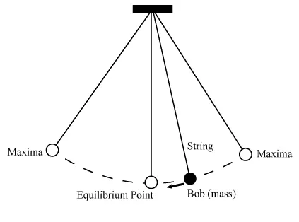
A simple pendulum is a mechanical arrangement that demonstrates periodic motion. The simple pendulum comprises a small bob of mass ‘m’ suspended by a thin string secured to a platform at its upper end of length 'l'.

The simple pendulum is a mechanical system that sways or moves in an oscillatory motion. This motion occurs in a vertical plane and is mainly driven by the gravitational force.

The length of the string is large compared to the dimensions of the bob. A stationary pendulum has its string in a vertical position with the bob hanging straight down. This is known as the pendulum's equilibrium position (since if left undisturbed, the pendulum will remain in this position). Oscillations (to and fro motion) are set up in a pendulum by displacing the bob from its equilibrium position and releasing it.

A second-order ordinary differential equation is an ordinary differential equation in which any derivatives with respect to the independent variable have order no greater than 2.

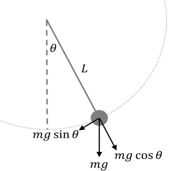
GOVERNING EQUATION:

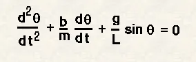
In the above equation,

g = gravity in m/s²,

L = length of the pendulum in m,

m = mass of the ball in kg,

b=damping coefficient.

For using the ode45 function we assume some relations:

ie.

assume θ=θ₁ ........................(1)

so, we can write dθ/dt = dθ₁/dt.................(2)

assume dθ₁/dt=θ₂..................(3)

so, we can write dθ/dt = dθ₁/dt=θ₂...................(4)

Therefore, d²θ/dt² = dθ₂/dt..................(5)

By using the following relations we write governing into,

dθ₂/dt = -(b/m)*θ₂ - (g/L) sin(θ₁)...................(6)

Values Given:

L=1 metre,

m=1 kg,

b=0.05.

g=9.81 m/s².

CODE FOR MATLAB:

1. Function Program

This program is coded using the equations 1 to 6.

Code:

function [dtheta_dt]=ode_func(t,theta,b,g,l,m)  %creates a function for solving ODE
theta1 = theta(1);  %define theta1 = theta(1).
theta2 = theta(2);  %define theta2 = theta(2).
dtheta1_dt = theta2;    %assumed dtheta1_dt = theta2
dtheta2_dt = -(b/m)*theta2 - (g/l)*sin(theta1); %creates this equation using above relations.
[dtheta_dt] = [dtheta1_dt; dtheta2_dt];   %creates matrix with first value as dtheta1_dt and second value as dtheta2_dt.
end     %end of the function

2. Main Program

We use ode45 for solving differential equations, the syntax we use in our problem is:

The general syntax is,

ode45(odefun,t_span,y0)

where t_span = [t0 tf], integrates the system of differential equations y′=f(t,y) from t0 to tf with initial conditions y0. Each row in the solution array y corresponds to a value returned in column vector t.

so in our case,

@(t,theta) means our function depends on (t,theta) these are main inputs in our ode.

ode_func means ode function and inside bracket consist of its variables

Instead of tspan we use t_span, it is a range of time values with initial condition 0 and final condition 20 sec.

And the differential equation is θ^’’ = f(t,θ)

Instead of y we use theta_0 which have two cases one is angular displacement and another one is angular velocity.

ie, integrates the system of differential equation θ^’’ = f(t,θ) from 0 to 20 with initial conditions theta_0. Each row in the solution array 'results' corresponds to a value returned in column vector

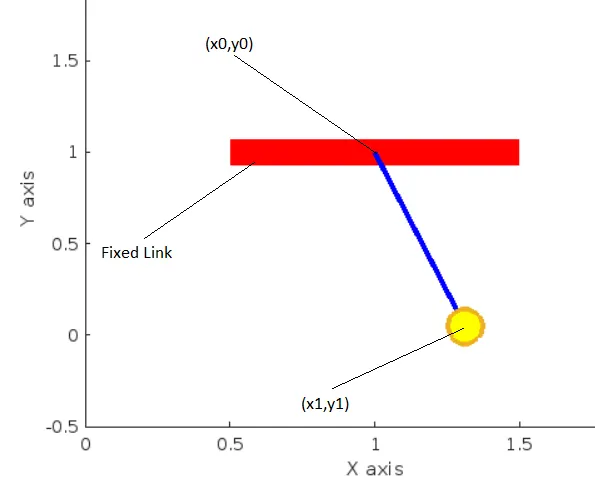
We create a fixed link with fixed point for oscillation of mass bob sphere,as shown in the figure

Fixed point

x0 = 1

y0 = 1

Centre of sphere

x1= x0 - l*sin(angular displacement)

y1 = y0 - l*cos(angular displacement)

Code:

clear all                           %clear the workspace if there any previus data exist.
close all                           %close all figures and plots
clc                                 %clear the command window if there any previus data exist.

% Variables used
b=0.05;         %damping coefficient 
g=9.81;         %gravity in [m/s^2]
l=1;            %length of the pendulum in [m]
m=1;            %mass of theball in [kg]

%intial condition
theta_0=[0;3]; %inital angular displacement and velocity are 0 [rad] and 3 [rad/s]

%time span
t_span=linspace(0,20,600); %motion time taken from 0 to 20 with 600 points.

%sole ODE
[t,results]=ode45(@(t,theta) ode_func(t,theta,b,g,l,m),t_span,theta_0); %calling ode function and we get t as column matrix with 600 terms ranges 
                                                                        % from 0 to 20, and we get results as 600*2 matrix with first column as 
                                                                        % displacement and second column refers velocity with 600 points 
                                                                    
figure(1)       %creates a figure
plot(t,results(:,1))    %plot a data series b/w time and displacement
hold on                 %retains plots in the current axes so that new plots added to the axes do not delete existing plots
plot(t,results(:,2))    %plot a data series b/w time and velocity
xlabel('Time (sec)')          %defines x axis as 'Time'
ylabel('Vel.(rad),& Disp.(rad/s)')          %defines y axis as 'Vel.(rad),& Disp.(rad/s)'.
legend('Angular Displacement','Angular Velocity')   %named first plotted data series as 'Angular Displacement' and 2nd as 'Angular Velocity'.
hold off    %using this we can stop use current axes properties for further step.

ang_disp = results(:,1);    %give 'results' first column as ang_disp
ang_vel = results(:,2);     %give 'results' second column as ang_vel

% giving values to fixed point on the fixed link
x0=1;   
y0=1;
ct=1;   %ct value is equal to 1. And it used for frame iteration purpose.

for i=1:length(ang_disp)    %for loop give i ranges from 1 to length of the ang_disp ie. 600 in this case.
    ang_disp1 = ang_disp(i);    %by changing the value of i, ang_disp1 take each value in each loop from the column matrix ang_disp
    x1=x0 - l*sin(ang_disp1);   %giving trignometric relation for defining x1 value
    y1=y0 - l*cos(ang_disp1);   %giving trignometric relation for defining y1 value

    figure(2)   %creates an another figure
    plot([0.5,1.5],[1,1],'-','linewidth',15,'color','r')    %plot a fixed link with coordinates (0.5,1) and (1.5,1)
    hold on %retains plots in the current axes so that new plots added to the axes do not delete existing plots
    plot([x0,x1],[y0,y1],'b-',x1,y1,'o','markersize',20,'markerfacecolor','y','linewidth',3) %plot a ine with points (x0,y0) and (x1,y1),
                                                                                             % and creates a sphere with face color yellow.
    axis([0 2 -.5 2]) %creates an axis with x axis ranges from 0 to 2, y axis ranges from -0.5 to 2
    xlabel('X axis')    %named x axis as 'X axis'.
    ylabel('Y axis')    %named y axis as 'Y axis'.
    title('Motion of a simple pendulum')    %named title as 'Motion of a simple pendulum'.
    M(ct) = getframe(gcf);  %captures the frame in loop manner
    ct = ct + 1;    %give a increment of +1 for ct value for next loop.
    hold off    %using this we can stop use current axes properties for further step.
end         %for loop ended.


movie(M)    %this command plays this as a movie with help of frames saved in M.
videofile = VideoWriter('Simple Pendulum','Uncompressed AVI');  %creates objects for the video with filename 
                                                                %in first place,& specified format in the 
                                                                %second place this is assigned to 'videfile'.
open(videofile)     %open the file that saved in videofile.
writeVideo(videofile,M) %writes objects into video with frame function M.
close(videofile)    %close the file videofile.


%Relation used in the function are based on the common procedure to solve a
%ODE problem using ode45

function [dtheta_dt]=ode_func(t,theta,b,g,l,m)  %creates a function for solving ODE
theta1 = theta(1);  %define theta1 = theta(1).
theta2 = theta(2);  %define theta2 = theta(2).
dtheta1_dt = theta2;    %assumed dtheta1_dt = theta2
dtheta2_dt = -(b/m)*theta2 - (g/l)*sin(theta1); %creates this equation using above relations.
[dtheta_dt] = [dtheta1_dt; dtheta2_dt];   %creates matrix with first value as dtheta1_dt and second value as dtheta2_dt.
end     %end of the function

OUTPUTS:

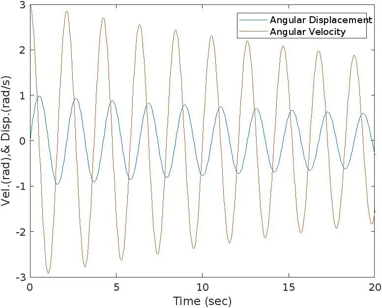
1. Graph

2. Animation Video

https://youtu.be/Gq32HZT0UVE

CONCLUSION:

1. Graph is plotted b/w time vs velocity, & displacement by solving the second ODE.

2. Animation video of the simple pendulum is created.

From the graph, we can identify that the amplitude of angular displacement and velocity decreases with respect to time,it is due to the damping effect.