Project 1 - Parsing NASA thermodynamic data
AIM: Parsing NASA thermodynamic data using MATLAB
OBJECTIVES:
1. Write a function that extracts the 14 co-efficients and calculates the enthalpy, entropy and specific heats for all the species in the data file
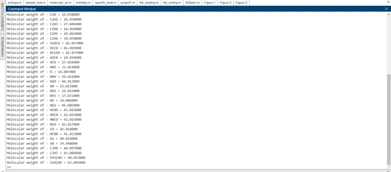
2. Calculate the molecular weight of each species.
3. Plot the Cp, Enthalpy and Entropy for the local temperature range, specific for each species.
4. Save the plots as images with appropriate names and dump them in separate folders for each species with suitable name.
5. Generate Cp, H and S plots.
THEORY:
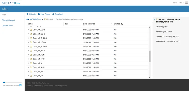
Definitions:
Enthalphy
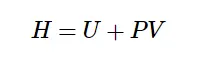
In thermodynamics, the enthalpy is the measure of energy in a thermodynamic system. It is the thermodynamic quantity equivalent to the total heat content of a system. The enthalpy is defined to be the sum of the internal energy E plus the product of the pressure p and volume V. In many thermodynamic analyses the sum of the internal energy U and the product of pressure p and volume V appears, therefore it is convenient to give the combination a name, enthalpy, and a distinct symbol, H.
H = U + pV
Entropy
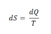
In thermodynamics and statistical physics, entropy is a quantitative measure of disorder, or of the energy in a system to do work.In statistical physics, entropy is a measure of the disorder of a system.The SI unit for entropy is J/K. According to Clausius, the entropy was defined via the change in entropy S of a system. The change in entropy S, when an amount of heat Q is added to it by a reversible process at constant temperature, is given by:
Specific Heat
Specific heat is a property related to internal energy that is very important in thermodynamics. The intensive properties cv and cp are defined for pure, simple compressible substances as partial derivatives of the internal energy u(T, v) and enthalpy h(T, p), respectively:
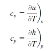
But we are considering cp in or problem.
File Parsing:
In our problem we have 53 species and each have 14 co-efficients. We use them calculates the enthalpy, entropy and specific heats for all the species in the data file. The formula are shown below.

Here R is the universal gas constant, T is the temperature.
The FIRST 7 coefficients are HIGH-temperature coefficients and the SECOND 7 coefficients are LOW-temperature coefficients.
Explanations:
1. Getting Header Information:
For reading the header information first we have to read the file by opening the data file 'THERMO.dat' using the fopen command, and r helps to read it. Then we use fgetl command with input as file name f1 that is previous assigned using fopen command.
Code:
clear all                           %clear the workspace if there any previus data exist.
close all                           %close all figures and plots
clc                                 %clear the command window if there any previus data exist.

%Reading datas from THERMO.dat file
f1 = fopen('THERMO.dat','r');   %read the file THERM.dat file
fgetl(f1);   %read the first line of THERMO.dat
2. Getting global temperature ranges:
Next line of the program is assign as temp using fgetl command, then we split the line string to different terms using strsplit command. So after all space it split the terms. Then we assign each terms as global temperature low, mid, and high. g{1} is not used because it is null string. And we use '{}' because it is string.
Code:
%Global temperature ranges
temp = fgetl(f1);   %assign the second line as temp
g = strsplit(temp); %strsplit used to split the string and allocate to g.

%assign the temperature value in global low,mid,high by converting string
%into number
global_low_temp = str2num(g{2});    %strnum used to convert string into number %Global low temperature
global_mid_temp = str2num(g{3});    %Global mid temperature
global_high_temp = str2num(g{4});   %Global high temperature
3. Skip the next three lines :
We use a for loop to skip the lines. And hide that datas using semicolon.
%skip next three lines
for i=1:3
    skip = fgetl(f1);
end
4. Extracting the local temperatures and coefficient values:
We use for loop for finding the 53 species. There are four lines of datas for each set of species , we name each line as tline1, tline2, tline3, and tline4. using fgetl command. Split the strings into different terms, and assign the first term as 'species'. And extract the local temperature range using str2num command. The local temperature ranges are positioned in same manner in each species, ie end-1, end-2, end-3 as high,mid,low temperatures respectively. (end means the last term)
Next three lines are coded in same manner, ie, first name the line using fgetl. There is common relation for every term, only three numbers are remain after 'E' term. So, we use findstr to get 'E' term in the line then join term by take '+3' in each term. And convert string into number using strnum.
eg. 2.56942078E+00
we select terms from starting and add relation c(1)+3, the value inside the bracket indicates term number. We find all 14 coefficients in this way.
Code:
    tline1 = fgetl(f1);  %first line of the set
    c = strsplit(tline1);    %split the strings
    species =  c{1};  %assign the first term as species

    %local temperature ranges
    low_temp = str2num(c{end-3});   %local low temperature
    mid_temp = str2num(c{end-2});   %local mid temperature
    high_temp = str2num(c{end-1});  %local high temperature

    %second line of the set
    tline2 = fgetl(f1);
    c = findstr(tline2,'E');    %find the 'E' in each coefficient
    a1 = tline2(1:c(1)+3);    %extract each coefficients from 1 to 5.
    a1 = str2num(a1);         %convert all coefficients string into numbers from 1 to 5.
    a2 = tline2(c(1)+4:c(2)+3);
    a2 = str2num(a2);
    a3 = tline2(c(2)+4:c(3)+3);
    a3 = str2num(a3);
    a4 = tline2(c(3)+4:c(4)+3);
    a4 = str2num(a4);
    a5 = tline2(c(4)+4:c(5)+3);
    a5 = str2num(a5);

    %third line of the set
    tline3 = fgetl(f1);
    d = findstr(tline3,'E');
    a6 = tline3(1:d(1)+3);  %extract each coefficients from 6 to 10.
    a6 = str2num(a6);       %convert all coefficients strings into numbers from 6 to 10.
    a7 = tline3(d(1)+4:d(2)+3);
    a7 = str2num(a7);
    a8 = tline3(d(2)+4:d(3)+3);
    a8 = str2num(a8);
    a9 = tline3(d(3)+4:d(4)+3);
    a9 = str2num(a9);
    a10 = tline3(d(4)+4:d(5)+3);
    a10 = str2num(a10);

    %fourth line of the set
    tline4 = fgetl(f1);
    e = findstr(tline3,'E');
    a11 = tline4(1:e(1)+3);     %extract each coefficients from 11 to 14.
    a11 = str2num(a11);         %convert all coefficients strings into numbers from 11 to 14.
    a12 = tline4(e(1)+4:e(2)+3);
    a12 = str2num(a12);
    a13 = tline4(e(2)+4:e(3)+3);
    a13 = str2num(a13);
    a14 = tline4(e(3)+4:e(4)+3);
    a14 = str2num(a14);
5. Specific heat calculation:
We create function with input variables a1, a2, a3, a4, a5, a8, a9, a10, a11, a12, t, mid_temp, R.
where,
a1, a2, a3, a4, a5 are high temperature coefficients
a8, a9, a10, a11, a12 are low temperature coefficients
t is local temperature range defined by linspace
mid_temp is the local mid temperature
R is the universal gas coefficient.
if - else condition helps to take high and low temperature ranges for calculation. If the condtion(t>=mid_temp) not satisfied it enters into the else loop.
For high temperature coefficients (t is take as values above local mid temperature).
For low temperature coefficients (t is take as values below local mid temperature).
Code:
function Cp = specific_heat(a1,a2,a3,a4,a5,a8,a9,a10,a11,a12,t,mid_temp,R)  %creating function

if t>=mid_temp      %if condition to high temp coefficents for calculation
    Cp = (a1 + a2*t + a3*(t).^2 + a4*(t).^3 + a5*(t).^4)*R;
else                %else this take low temp coefficients for calculation
    Cp = (a8 + a9*t + a10*(t).^2 + a11*(t).^3 + a12*(t).^4)*R;
end
6. Enthalphy calculation:
We create function with input variables a1, a2, a3, a4, a5, a6, a8, a9, a10, a11, a12, a13, t, mid_temp, R.
where,
a1, a2, a3, a4, a5, a6 are high temperature coefficients
a8, a9, a10, a11, a12, a13 are low temperature coefficients
t is local temperature range defined by linspace
mid_temp is the local mid temperature
R is the universal gas coefficient.
if - else condition helps to take high and low temperature ranges for calculation. If the condtion(t>=mid_temp) not satisfied it enters into the else loop.
For high temperature coefficients (t is take as values above local mid temperature).
For low temperature coefficients (t is take as values below local mid temperature).
Code:
function H = enthalpy(a1,a2,a3,a4,a5,a6,a8,a9,a10,a11,a12,a13,t,mid_temp,R)     %creating function

if t>=mid_temp    %if condition to high temp coefficents for calculation
    H = (a1 + ((a2.*t)./2) + ((a3.*(t).^2)./3) + ((a4.*(t).^3)./4) + ((a5.*(t).^4)./5) + (a6./t)).*R.*t;
else              %else this take low temp coefficients for calculation
    H = (a8 + ((a9.*t)./2) + ((a10.*(t).^2)./3) + ((a11.*(t).^3)./4) + ((a12.*(t).^4)./5) + (a13./t)).*R.*t;
end
7. Entropy calculation:
We create function with input variables a1, a2, a3, a4, a5, a7, a8, a9, a10, a11, a12, a14, t, mid_temp, R.
where,
a1, a2, a3, a4, a5, a7 are high temperature coefficients
a8, a9, a10, a11, a12, a14 are low temperature coefficients
t is local temperature range defined by linspace
mid_temp is the local mid temperature
R is the universal gas coefficient.
if - else condition helps to take high and low temperature ranges for calculation. If the condtion(t>=mid_temp) not satisfied it enters into the else loop.
For high temperature coefficients (t is take as values above local mid temperature).
For low temperature coefficients (t is take as values below local mid temperature).
Code:
function S = entropy(a1,a2,a3,a4,a5,a7,a8,a9,a10,a11,a12,a14,t,mid_temp,R)  %creating function

if t>=mid_temp      %if condition to high temp coefficents for calculation
    S = ((a1*log(t)) + (a2*t) + (a3*(t).^2)/2 + (a4*(t).^3)/3 + (a5*(t).^4)/4 + (a7))*R;
else                %else this take low temp coefficients for calculation
    S = ((a8*log(t)) + (a9*t) + (a10*(t).^2)/2 + (a11*(t).^3)/3 + (a12*(t).^4)/4 + (a14))*R;
end
8. Molecular weight calculation:
We create a function for finding the molecular weight of species. First, we define elements that are commonly used species. And we define the corresponding atomic weight of the element. mol_wt is value as zero for calculation purpose. Next we create for loops, first for loop for taking species elements one by one and second for loop used take element from the elements. Two strings are compared using the strcmpi command. If it matches, it take corresponding atomic weight and add up in the equation. If it doesn't match it should be a number, so first convert the string into number using strnum this value is assign to n. And if the number is greater than 1, then it equate into the last equation.
eg. H2O
First element 'H' matches with elements, and it matches with elements(1) ie, j=1. So our current mol_wt becomes 1.008. Then second term '2' runs in strcmpi but doesn't match with any of term in elements. So it enters to strnum, it convert the string into number. Then, it enters if that evaluates with expression n>1. Our n is 2 it greater than 1, then mol_wt = 1.008 + (1.008*(2-1)) where z = 1. Similarly 'O' is evaluated and mol_wt becomes 2.016+15.999 ie, 18.015.
Code:
function molecular_weight = molecular_wt(species)   %creating function
elements = ['H','C','O','N','A','S'];       %make an array for atoms
atomic_weight = [1.008 12.011 15.999 14.007 39.948 32.06];  %make an array of corresponding atomic weight
mol_wt = 0;    %assign mol_wt value as zero
for i = 1:length(species)
    for j = 1:length(elements)
        if strcmpi(species(i),elements(j))   %compare elements and atomic_weight string
        mol_wt = mol_wt + atomic_weight(j);
        z = j;
        end
    end
    n = str2num(species(i));    %species contain number as strings are converted into numerical number.
    if (n>1)
        mol_wt = mol_wt + (atomic_weight(z)*(n-1));
    end
    molecular_weight = mol_wt;
end
9. Create separate folders for each species:
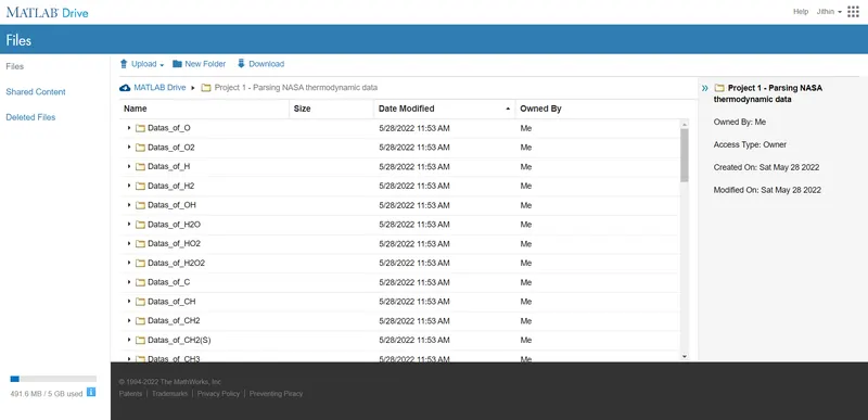
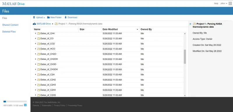
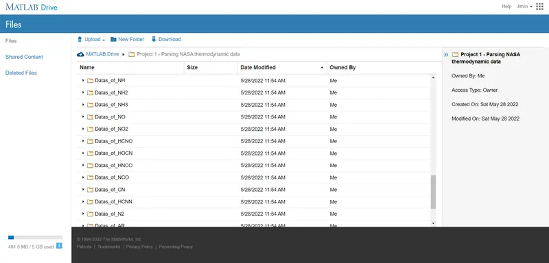
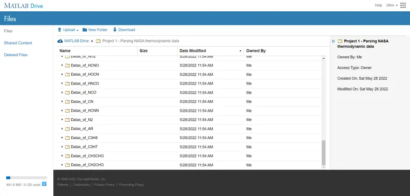
strcat - concatenate strings horizontally ie, first 'Datas_of_ ' then species name. Makes a new folder with name created by strcat using command mkdir. pwd identify current folder and displays in command box as 'file ='.
eg. O
'Datas_of_O' folder is created.
Code:
   %Create separate folders for each species
    data = strcat('Datas_of_ ',species);    %name the string horizontally
    mkdir(data)     %make the data assigned name as new folder
    file  = pwd;    %identify current folder
10. Plotting:
Each graph created in each figures using figure command. strcat used to name the title. fullfile creates full path to the folder. cd changes the current folder to a local folder 'Datas_of_'species. Then save the plot as png in that folder with specific name. Then return the folder to the path that is defined to file (cd(file)). gcf command is used to handel the current figures. All figures using same format.
eg: O
plot the graph and save in the folder '/MATLAB Drive/Project 1 - Parsing NASA thermodynamic data/Datas_of_O' in png format. And returns to the folder '/MATLAB Drive/Project 1 - Parsing NASA thermodynamic data'.
Note: cd(file) is very important to store datas of each species in different folder in the home folder 'Project 1 - Parsing NASA thermodynamic data'.
Code:
    %plotting figure 1
    figure(1)   %creates figure 1
    plot(Cp,t,'-r')     %plot the graph with red line.
    data1 = strcat(species,' - Specific Heat vs Temperature Graph');    %name the string horizonatlly
    xlabel('Specific Heat') %naming x-axis
    ylabel('Temperature')   %naming y-axis
    title(data1)    %naming title
    grid on     %turn the grids on
    f = fullfile(data); %bulid a full name for the folder
    cd(f)   %change the folder to 'f'.
    saveas(gcf,[pwd '/Specific Heat vs Temperature Graph.png']) %save the graph as png in that folder.
    cd(file)    %return folder path to home folder.

    %plotting figure 2
    figure(2)       %creates figure 2.
    plot(H,t,'-b')      %plot the graph with blue line.
    data2 = strcat(species,' - Enthalphy vs Temperature Graph');    %name the string horizonatlly
    xlabel('Enthalphy')     %naming x-axis
    ylabel('Temperature')   %naming y-axis
    title(data2)    %naming title
    grid on     %turn the grids on
    f = fullfile(data);     %bulid a full name for the folder
    cd(f)
    saveas(gcf,[pwd '/Enthalphy vs Temperature Graph.png'])
    cd(file)

    %plotting figure 3
    figure(3)       %creates figure 3.
    plot(S,t,'-g')       %plot the graph with blue line.
    data3 = strcat(species,' - Entropy vs Temperature Graph');  %name the string horizonatlly
    xlabel('Entropy')   %naming x-axis
    ylabel('Temperature')   %naming y-axis
    title(data3)    %naming title
    grid on     %turn the grids on
    f = fullfile(data);     %bulid a full name for the folder
    cd(f)   %change the folder to 'f'.
    saveas(gcf,[pwd '/Entropy vs Temperature Graph.png'])   %save the graph as png in that folder.
    cd(file)    %return folder path to home folder.
MAIN PROGRAM:
clear all                           %clear the workspace if there any previus data exist.
close all                           %close all figures and plots
clc                                 %clear the command window if there any previus data exist.

%Reading datas from THERMO.dat file
f1 = fopen('THERMO.dat','r');   %read the file THERM.dat file
fgetl(f1);   %read the first line of THERMO.dat

%Global temperature ranges
temp = fgetl(f1);   %assign the second line as temp
g = strsplit(temp); %strsplit used to split the string and allocate to g.

%assign the temperature value in global low,mid,high by converting string
%into number
global_low_temp = str2num(g{2});    %strnum used to convert string into number %Global low temperature
global_mid_temp = str2num(g{3});    %Global mid temperature
global_high_temp = str2num(g{4});   %Global high temperature

%skip next three lines
for i=1:3
    skip = fgetl(f1);
end

%making for loop from next line onwards
for j = 1:53    %there 53 sets of species
    tline1 = fgetl(f1);  %first line of the set
    c = strsplit(tline1);    %split the strings
    species =  c{1};  %assign the first term as species

    %local temperature ranges
    low_temp = str2num(c{end-3});   %local low temperature
    mid_temp = str2num(c{end-2});   %local mid temperature
    high_temp = str2num(c{end-1});  %local high temperature

    %second line of the set
    tline2 = fgetl(f1);
    c = findstr(tline2,'E');    %find the 'E' in each coefficient
    a1 = tline2(1:c(1)+3);    %extract each coefficients from 1 to 5.
    a1 = str2num(a1);         %convert all coefficients string into numbers from 1 to 5.
    a2 = tline2(c(1)+4:c(2)+3);
    a2 = str2num(a2);
    a3 = tline2(c(2)+4:c(3)+3);
    a3 = str2num(a3);
    a4 = tline2(c(3)+4:c(4)+3);
    a4 = str2num(a4);
    a5 = tline2(c(4)+4:c(5)+3);
    a5 = str2num(a5);

    %third line of the set
    tline3 = fgetl(f1);
    d = findstr(tline3,'E');
    a6 = tline3(1:d(1)+3);  %extract each coefficients from 6 to 10.
    a6 = str2num(a6);       %convert all coefficients strings into numbers from 6 to 10.
    a7 = tline3(d(1)+4:d(2)+3);
    a7 = str2num(a7);
    a8 = tline3(d(2)+4:d(3)+3);
    a8 = str2num(a8);
    a9 = tline3(d(3)+4:d(4)+3);
    a9 = str2num(a9);
    a10 = tline3(d(4)+4:d(5)+3);
    a10 = str2num(a10);

    %fourth line of the set
    tline4 = fgetl(f1);
    e = findstr(tline3,'E');
    a11 = tline4(1:e(1)+3);     %extract each coefficients from 11 to 14.
    a11 = str2num(a11);         %convert all coefficients strings into numbers from 11 to 14.
    a12 = tline4(e(1)+4:e(2)+3);
    a12 = str2num(a12);
    a13 = tline4(e(2)+4:e(3)+3);
    a13 = str2num(a13);
    a14 = tline4(e(3)+4:e(4)+3);
    a14 = str2num(a14);

    %Universal Gas Constant [J/Kmol]
    R = 8.31446261815324;

    %Local temperature range for calulation
    t = linspace(low_temp,high_temp,500);   %making an array of temperatures from local low temp to local high temp with 500 points.

    %specific heat [J/kgK]
    Cp = specific_heat(a1,a2,a3,a4,a5,a8,a9,a10,a11,a12,t,mid_temp,R);  %Calling specific_heat function

    %Enthalpy [J/kg]
    H = enthalpy(a1,a2,a3,a4,a5,a6,a8,a9,a10,a11,a12,a13,t,mid_temp,R);     %calling enthalphy function

    %Entropy [J/K]
    S = entropy(a1,a2,a3,a4,a5,a7,a8,a9,a10,a11,a12,a14,t,mid_temp,R);  %calling entropy function

    % Molecular weight [g/mol]
    molecular_weight = molecular_wt(species);    %calling molecular_wt function
    h = sprintf('Molecular weight of - %s = %f',species,molecular_weight);  %format the datas into character vector
    disp(h)     %display character in the command box

   %Create separate folders for each species
    data = strcat('Datas_of_ ',species);    %name the string horizontally
    mkdir(data)     %make the data assigned name as new folder
    file  = pwd;    %identify current folder

    %plotting figure 1
    figure(1)   %creates figure 1
    plot(Cp,t,'-r')     %plot the graph with red line.
    data1 = strcat(species,' - Specific Heat vs Temperature Graph');    %name the string horizonatlly
    xlabel('Specific Heat') %naming x-axis
    ylabel('Temperature')   %naming y-axis
    title(data1)    %naming title
    grid on     %turn the grids on
    f = fullfile(data); %bulid a full name for the folder
    cd(f)   %change the folder to 'f'.
    saveas(gcf,[pwd '/Specific Heat vs Temperature Graph.png']) %save the graph as png in that folder.
    cd(file)    %return folder path to home folder.

    %plotting figure 2
    figure(2)       %creates figure 2.
    plot(H,t,'-b')      %plot the graph with blue line.
    data2 = strcat(species,' - Enthalphy vs Temperature Graph');    %name the string horizonatlly
    xlabel('Enthalphy')     %naming x-axis
    ylabel('Temperature')   %naming y-axis
    title(data2)    %naming title
    grid on     %turn the grids on
    f = fullfile(data);     %bulid a full name for the folder
    cd(f)
    saveas(gcf,[pwd '/Enthalphy vs Temperature Graph.png'])
    cd(file)

    %plotting figure 3
    figure(3)       %creates figure 3.
    plot(S,t,'-g')       %plot the graph with blue line.
    data3 = strcat(species,' - Entropy vs Temperature Graph');  %name the string horizonatlly
    xlabel('Entropy')   %naming x-axis
    ylabel('Temperature')   %naming y-axis
    title(data3)    %naming title
    grid on     %turn the grids on
    f = fullfile(data);     %bulid a full name for the folder
    cd(f)   %change the folder to 'f'.
    saveas(gcf,[pwd '/Entropy vs Temperature Graph.png'])   %save the graph as png in that folder.
    cd(file)    %return folder path to home folder.

end

fclose(f1);
SCREENSHOTS:
Folders:
Molecular Weight:
PLOTS:
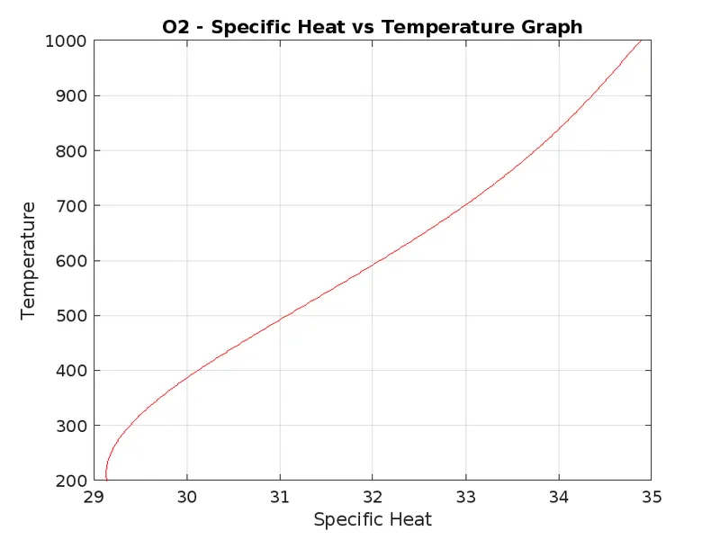
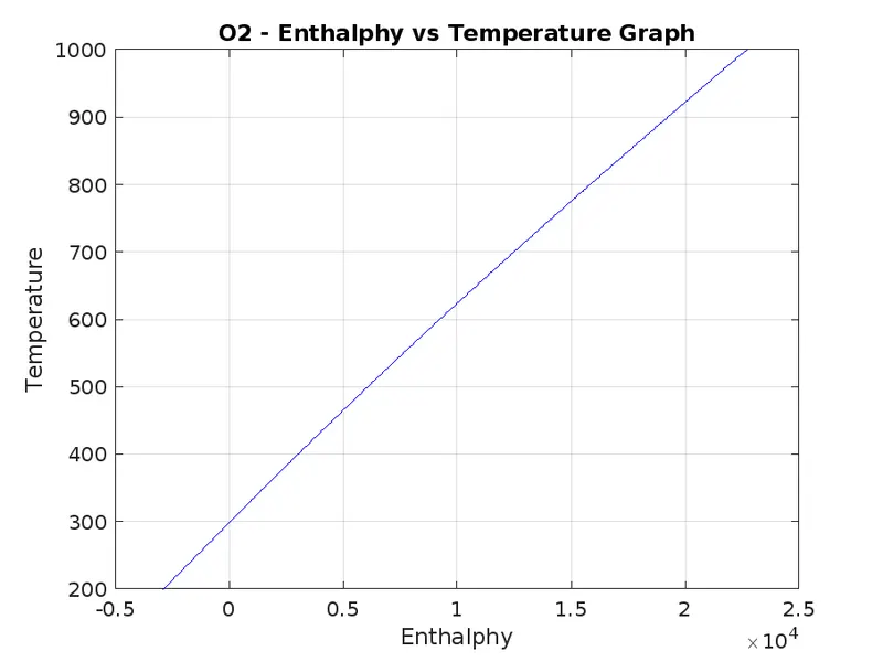
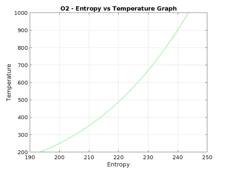
Molecular Oxygen (O2):
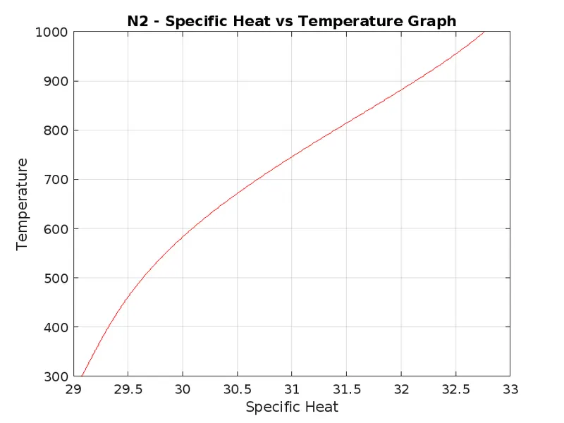
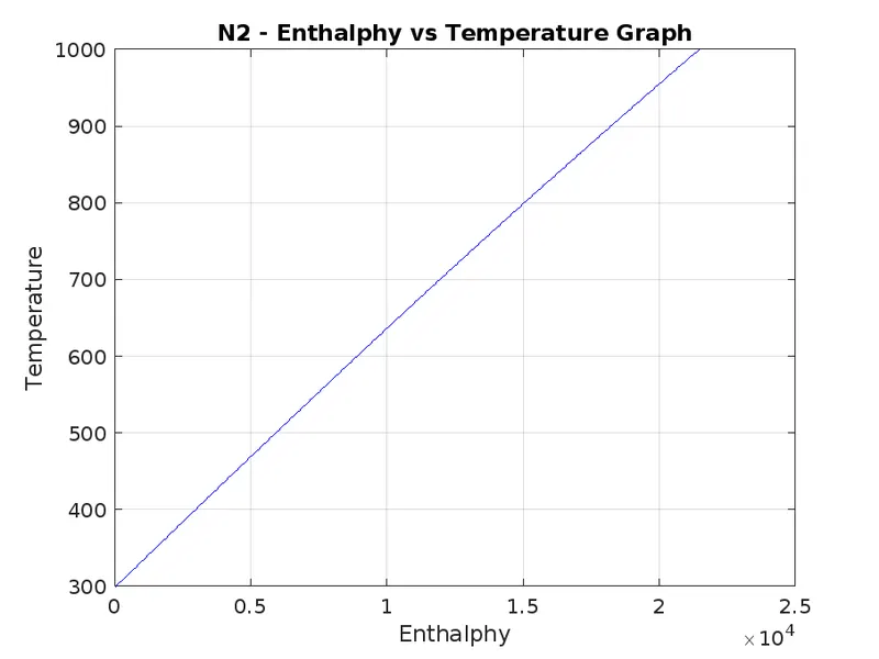
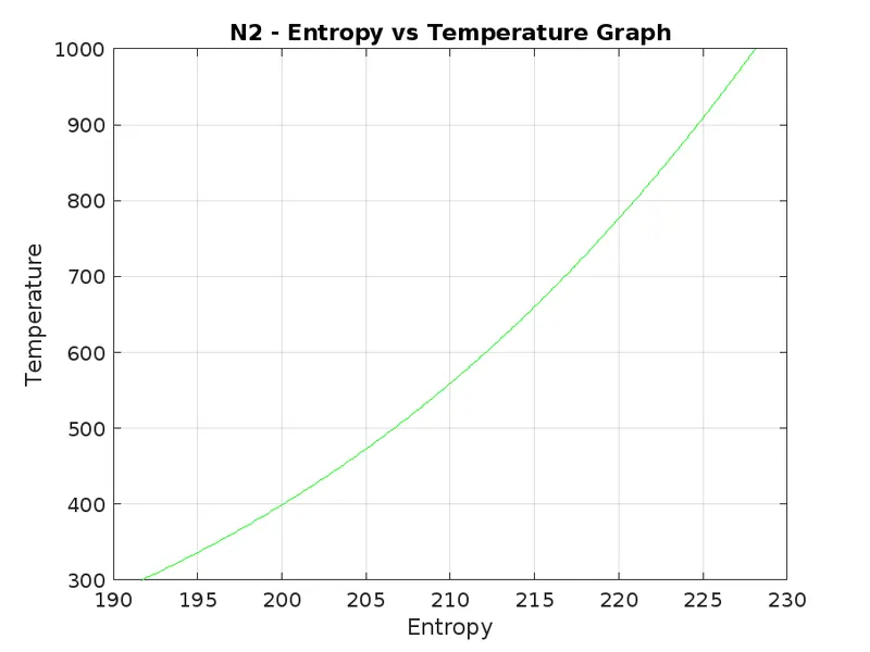
Molecular Nitrogen (N2):
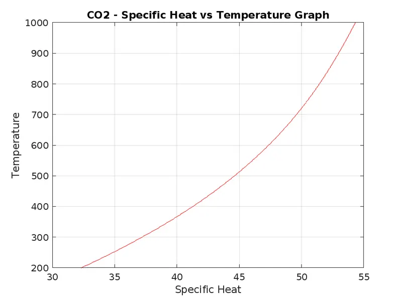
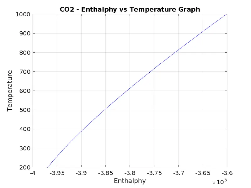
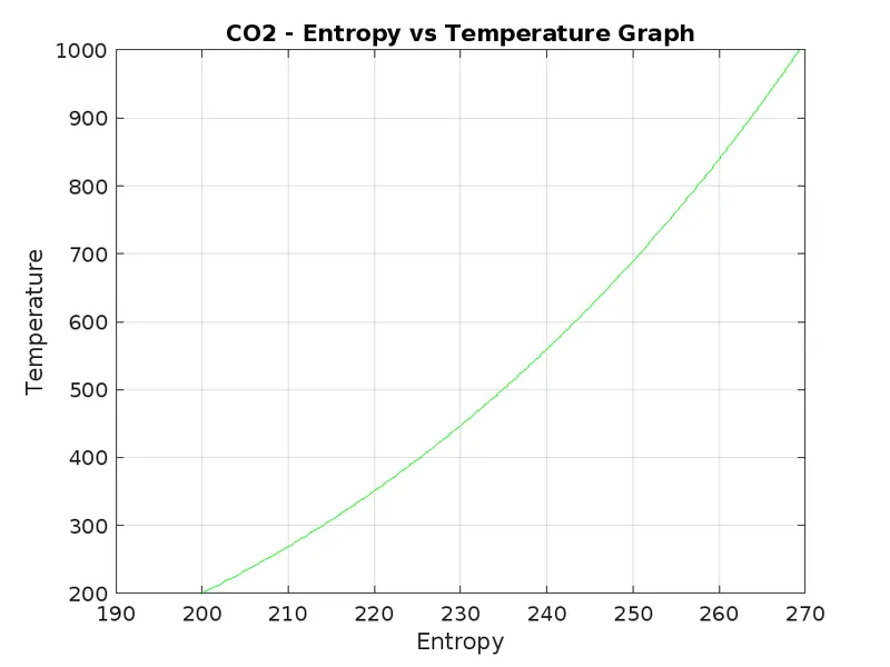
Carbon Dioxide (CO2):
CONCLUSIONS:
- The datas are extracted from THERMO.dat file and finded specific heat, enthalphy, entropy, molecular weight.
- Plotted graphs corresponding to each species. And arranged the datas of each species in different folder.
Specific heat vs Temperature Graph
Specific heat of substance increases with increase in temperature.At ordinary temperatures, specific heat increase only slowly as temperature increases. For many purposes they can be taken to be constant over rather wide temperature ranges.
Enthalphy vs Temperature Graph
When the number of interactions increase, then the internal energy of the system rises. According to the first equation given, if the internal energy (U) increases then the ΔH increases as temperature rises.
Entropy vs Temperature Graph
If you increase temperature, you increase entropy. More energy put into a system excites the molecules and the amount of random activity. Since entropy is the quantity of disorderness in the system, entropy of the system increases.