Challenge

Week 4.1 - Genetic Algorithm

PPratik Dhokale20 May 2022

Week 4.1 - Genetic Algorithm

Aim:

Write a code in MATLAB to optimise the stalagmite function and find the global maxima of the function.
Plot graphs for all 3 studies and for F maximum vs no. of iterations.

Theory

Genetic algorithm is process of solving optimization problems based on natural selection and that drives biological evolution. The approach to optimization is based on the concept of survival of the fittest. In such process, strogest elements become stronger and weakest elements are eliminated.

The following outline summarizes how the genetic algorithm works:

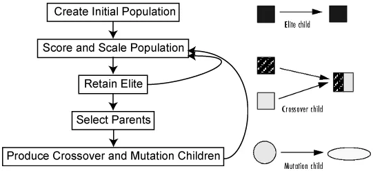
The algorithm begins by creating a random initial population.
The algorithm then creates a sequence of new populations. At each step, the algorithm uses the individuals in the current generation to create the next population. To create the new population, the algorithm performs the following steps:
1. Scores each member of the current population by computing its fitness value. These values are called the raw fitness scores.
2. The algorithm involves retaining the best individuals for the next population. The other individuals are replaced by new individuals formed through processes of crossover and mutation.
3. Some of the individuals in the current population that have lower fitness are chosen as elite. These elite individuals are passed to the next population.
4. Produces children from the parents. Children are produced either by making random changes to a single parent- mutation or by combining the vector entries of a pair of parents- crossover.
5. Crossover is a process in which two indivduals from the current generation engage in a procedure in which some genes from one parent are interchanged with genes from the corresponding positions in the other. This process produces two new individuals
6. Mutation involves selection, on a random basis, of a certain number of the genes in the current population and random alterations are then made to their values.
7. Replaces the current population with the children to form the next generation.
The algorithm stops when one of the following stopping criteria is met (See the default values for each option by running opts=optimoptions('ga'))
- MaxGenerations- The algorithm stops when the number of generations reaches MaxGenerationsThe algorithm stops after running for an amount of time in seconds equal to MaxTime
- FitnessLimit — The algorithm stops when the value of the fitness function for the best point in the current population is less than or equal to FitnessLimit.
- MaxStallGenerations — The algorithm stops when the average relative change in the fitness function value over MaxStallGenerations is less than Function tolerance.
- MaxStallTime — The algorithm stops if there is no improvement in the objective function during an interval of time in seconds equal to MaxStallTime.
- FunctionTolerance — The algorithm runs until the average relative change in the fitness function value over MaxStallGenerations is less than Function tolerance.
- ConstraintTolerance — The ConstraintTolerance is not used as stopping criterion. It is used to determine the feasibility with respect to nonlinear constraints. Also, max(sqrt(eps),ConstraintTolerance) determines feasibility with respect to linear constraints.

Syntax for ga

ga- is used to find minimum of function using Genetic algorithm

x=ga(fun,nvars)
finds a local unconstrained minimum, x, to the objective function,fun. nvars is the dimension (number of design variables) of fun
x=ga(fun,nvars,A,b,Aeq,beq,lb,ub,nonlcon,IntCon,options)
A,b- Linear inequality constraints `A*xleb`
Aeq,beq- Linear equality constraints `Aeq*xlebeq`
lb- lower bound limit
ub- Upper bound limit
nonlcon- Non linear constraints, specified as function handle
IntCon- Integer variables, specified as a vector of positive integers taking values from 1 to nvars
options- used to define new population size by minimizing default value created using optimoptions.
for no no bounds and no nonlinear equalities/ constraints use [].

Stalagmite function
Here we writing a code for optimization stalagmite function and find the global maxima of the function.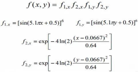

Seperate function is created with all these equations and later it is called in ga program to find global maxima. GA gives the minimum of function so to find maxima of function, function is given negative sign. The code for the function is as below-

%% Week 4.1- Genetic Algorithm

function [f]=stalagmite(input_vector)

x=input_vector(1);
y=input_vector(2);

% Stalagmite functions
f1x=(sin(5.1*pi*x+0.5)).^6;
f1y=(sin(5.1*pi*y+0.5)).^6;

f2x=exp(-4*log(2)*((x-0.0667).^2)/0.64);
f2y=exp(-4*log(2)*((y-0.0667).^2)/0.64);

f=-(f1x.*f2x.*f1y.*f2y);   % '-'ve sign to find max of function
end

GA code to find global maxima

First, clear all, close all and clc is used to erase previous data.
Search space is defined using linspace command and the it converted into 2D mesh using meshgrid(x,y) command.
Defined no of iterations.
For loop is used to find optimum value at each meshgrid point to evaluate stalagmite function. Iterations for this loop are equal to the length of meshgrid. Stalagmite function created earlier is called here.
Using surf command this contour surface of this stalagmite function is created. And mesh lines are removed using shading interp command. To generate maxima of function negative sign is given to the function.
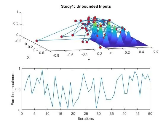
Study 1
In this study of statistical behavior without bounded inputs, optimum value of function is calculated at each iteration and total iterations are equal to no of cases.
For loop is created to evaluate unconstrained max fun val at random 50 iteration. ga(fun,nvars) is used to calculate optimum fun value. And it's location saved as xop1 and yop1.
using tic and toc command study time is calculated.
To see results new figure is created. Stalagmite fun is plotted using surf command. Hold on command is used to retain stalagmite fun and 3d plot of optimum fun using plot3(x,y,z) command. Title and labels are provided to the content in the figure.
using subplot command Function and iteration graph is plotted and labelled. negative sign is given to find maximum value.
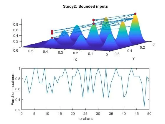
Study 2
In this study, upper and lower bounds are provided in ga function between 0 to 1. As no linear inequalities exists A,b,Aeq,beq=[].
optimum fun and its location is saved as fop2, xop2, yop2. And same graphs are plotted as per study 1. And study time is calculated.
Study 3
In this study, population size is increased to 500 using options and optimoptions command to minimize default value.
Graphs and surface contour are plotted and labelled as described previously.

fmax and input vector are calculate for this population using ga command.
Below is the final code for the same

%% Week 4.1- Genetic algorithm
clear all
close all
clc

%% Defining search space
x=linspace(0,0.6,150);      % x input
y=linspace(0,0.6,150);      % y input
no_cs=50;                   % No of iterations
[xx yy]=meshgrid(x,y);      % Creating 2D mesh

%% Evaluating the stalagmite function
for i=1:length(xx)
    for j=1:length(yy)
        input_vector(1)=xx(i,j);
        input_vector(2)=yy(i,j);
        f(i,j)=stalagmite(input_vector);
    end
end

%% Study 1- statistical behavior
tic                         % Study time start
for i=1:no_cs
    [res1,fop1(i)]=ga(@stalagmite,2);   % To find unconstrained max fun
    xop1(i)=res1(1);
    yop1(i)=res1(2);
end

study1_time=toc             % Study time stop

% Plotting
figure('Name','Study 1')    
subplot(2,1,1)              % location of 1st graphs in same figure
hold on                     % To retain the frames
surf(xx,yy,-f)              % Stalagmite function
shading interp              % Remove mesh line
plot3(xop1,yop1,-fop1,'marker','o','MarkerFaceColor','r')   % 3D Plot
title('Study1: Unbounded Inputs')   % Title of figure
xlabel('X')                 % X-axis label
ylabel('Y')                 % Y-axis label

subplot(2,1,2)              % Location of 2nd graph
plot(-fop1)                 % Function plot
xlabel('Iterations')
ylabel('Function maximum')

%% Study 2- Statistical behavior- with upper & lower bounds
tic                         % Study time start
for i=1:no_cs
    [res2,fop2(i)]=ga(@stalagmite,2,[],[],[],[],[0:0],[1:1]);
    % Above line defines set of lower and upper bounds to find solution in
    % between range. A,b,Aeq,beq=[] as no linear inequalities exist
    xop2(i)=res2(1);
    yop2(i)=res2(1);
end
study2_time=toc             % Study time stop

figure('Name','Study2')
subplot(2,1,1)
hold on
surfc(xx,yy,-f)
shading interp
plot3(xop2,yop2,-fop2, 'marker','o','MarkerFaceColor','r')
title('Study2: Bounded inputs')
xlabel('X')
ylabel('Y')

subplot(2,1,2)
plot(-fop2)
xlabel('Iterations')
ylabel('Function maximum')

%% Study 3- Increasing GA iterations

options=optimoptions('ga');     % returns a set of default options for the solver
options=optimoptions(options,'PopulationSize',500);     
% increase the population size to 500

tic                         % Study time start
for i=1:no_cs
    [res3,fop3(i)]=ga(@stalagmite,2,[],[],[],[],[0:0],[1:1],[],[],options);
    % [] for no nonlinear constraints. minimizes with the default
    % optimization parameter replaced by values in option
    xop3(i)=res3(1);
    yop3(i)=res3(1);
end
study3_time=toc             % Study time stop

figure('Name','Study3')
subplot(2,1,1)
hold on
surfc(xx,yy,-f)
shading interp
plot3(xop3,yop3,-fop3, 'marker','o','MarkerFaceColor','r')
title('Study3:Bounded inputs with modified population size')
xlabel('X')
ylabel('Y')

subplot(2,1,2)
plot(-fop3)
xlabel('Iterations')
ylabel('Function maximum')
[xy,fmax]=ga(@stalagmite,2,[],[],[],[],[0:0],[1:1],[],[],options)

Outputs

Study 1- Unbounded Inputs

Study1 time=3.25
Study 2- Bounded Inputs

Study2 time=3.51
Study 3- Bounded inputs with modified population size

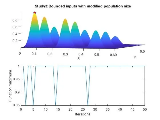
Study3 time=23.3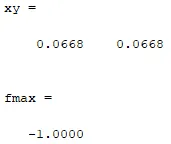

Conclusions

From the study 1, optimum fun val lies between 0 to 1. and giving lot of variation. Function doesn't recognise the search space. Due to random iterations and spread optimum value we cann't get max val of function
To overcome problem fun not recognising search space, in study 2 we provide bounded limits in ga code, because of bouded limits function is within search space and its value is between 0.4 to 1. From this we can say that by giving bounded limits variation in optimum val of function and can be reduced can be brought in within search space.
To get better desired value, ga is provided with bounded limits and increased population size in study 3, because of which we get less variation in optimum value. Increase in population value has led to give better fitness of the function and can give global maxima but at the same time it increases the study time.
Significance of running multiple iterations
If single iterations is done then we get different value at every time we run the program, so we cannot get the global maxima or minima. By running multiple iteraions we can increased the search space and desired range to find global maxima. From this study it is clear that if we do multiple iterations with bounded limits and increase population we can get only 1 desired optimum value.

Errors

There were few small typo errors in the code, which were corrected immediately. Surface plot for stalagmite function wasn't showing in study 1, realised that hold on command was missing.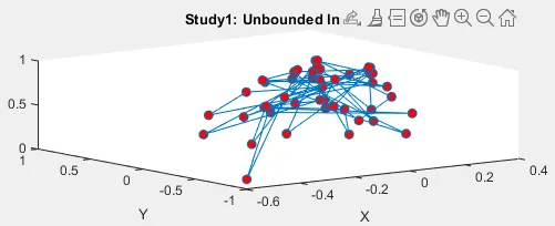

References

Week 4.1 - Genetic Algorithm

Ship work like this
in your own course.

Talk to a career counsellor

Ship work like thisin your own course.

Talk to a career counsellor

Ship work like this
in your own course.