Project 2 - Rankine cycle Simulator
Project 2- Rankine Cycle Simulator
AIM
- Create a Rankine Cycle Simulator using MATLAB
- Calculate the state points of the Rankine cycle based on user inputs.
- Plot the corresponding T-s & h-s plots for given set of inputs.
- Calculate Net work output & Back work ratio
THEORY
The Rankine cycle is an idealized thermodynamic cycle describing the process by which certain steam turbines or reciprocating steam engines, allow mechanical work to be extracted from a fluid as it moves beetween a heat source and heat sink. This cycle is named after William John Macquorn Rankine.
This method is widely used by power plants such as coal-fired power plants or nuclear power reactors. Heat energy is supplied to the system via boiler where the working fluid (typically water) is converted to a high pressure gaseous state (steam) in oreder to run a turbine. After passing over turbine the fluid is allowed to condense back into a liquid state as waste heat energy is rejected before being returned to boiler, completing the cycle. This cycle generally operate in a closed loop where the working fluid is reused.
Rankine cycle process
See the arrangement of a thermal power plant cycle in following figure. In ideal Rankine cycle, the system has four components and four processes.
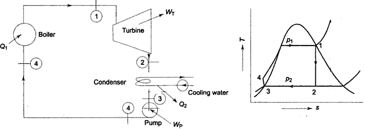
- Process 1-2: Isentropic expansion in Turbine
the dry saturated Steam will enter in to the turbine at high pressure and temp at point 1 and it will be expanded here. Due to expansion, we will have work output from turbine Wt and steam will be rejected as wet steam at low pressure and temperature at point 2.
`Wt=H1-H2` - Process 2-3: Isobaric Heat rejection in Condensor
At point 2 steam is in wet condition, this steam will enter condenser. Cooling water inside condenser will take away latent heat of wet steam and cool down steam. So at point 3, steam will leave condenser in a state of saturated liquid. This process will be steady flow process, hence pressure and temp will be constant throughout the process. Working fluid is rejecting heat energy Qout to the condenser during this process. This Heat rejected will be given by,
`Qout=H2-H3` - Process 3-4: Isentropic compression in Pump
Saturated liquid leaving the condenser will enter to the feed pump at lower pressure and temp at point 3. Pump will deliver the liquid water to the boiler at higher pressure with small rise in temp. In this process work will be done here on the system in order to pump the liquid at higher pressure.
`Wp=H4-H3` - Process 4-1: Isobaric heat addition in Boiler
High pressure liquid water will enter to the boiler at point 4. Heat energy is supplied to the water, this heat will convert water into dry saturated or superheated steam. So this process is constant pressure heat addition in boiler. Heat added Qin is given by
`Qtext(in)=H1-H4`
Other Thermodynamic equations
- Vapour fraction (x) at point 2
Entropy s2 at point 2 is given by
`s2=text(sf2)+x2.text(sfg)=text(sf2)+x2.(text(sg2-sf2))`
`therefore x2=(s2-text(sf2))/(sg2-text(sf2))` - Enthalpy h2 at point 2
`h2=hf2+x2*(hg2-hf2)` - T4 for isentropic process
`(T4)/(T3)=((P4)/(P3))^((1-1/gamma)`
`:. T4=T3*((P4)/(P3))^((1-1/gamma)`
`where..gamma=(cp4)/(cv4)` - Net work done
`text(wnet)=wt-wp` - Thermal efficiency `eta`
`eta=text(qin-qout)/text(qin)=(h1-h4+h2-h3)/(text(qin))=(wt-wp)/(text(qin))=text(wnet)/text(qin)` - Back work ratio
`bwr=text(Pump work)/text(Turbine work)=(wp)/(wt)` - Steam rate (SSC)
`ssc=text(mass flow rate)/text(Net work done)=3600/text(wnet)`
Required Inputs for Program
Turbine Inlet temperature = 400° C
Turbine Inlet Pressure = 30 bars
Turbine Outlet Pressure = 0.05 bars = Condenser Inlet Pressure
MAIN MATLAB PROGRAM
% Project 2- Rankine Cycle Simulator
clear all
close all
clc

%% Display Process
fprintf('\t\t\t\t\tRANKINE CYCLE SIMULATOR \n\n');
disp(' 1-2 is Isentropic Expansion in the Turbine');
disp(' 2-3 is Constanst Pressure Heat rejection by the Condensor');
disp(' 3-4 is Isentropic Compression in the Pump');
disp(' 4-1 is Const Pressure Heat Addition by the Boiler');
fprintf('\n');
%% Input from the user
P1=input('Enter the Pressure at the Turbine Inlet (in bar):');
T1=input('Enter the Temperature at the Turbine Inlet (in °C):');
P2=input('Enter the Pressure at the Condenser (in bar):');

%% Calculations
% State point 1
h1=XSteam('h_pT',P1,T1);        % Enthalpy at P1 & T1
s1=XSteam('s_pT',P1,T1);        % Entropy at P1 & T1

% State point 3
P3=P2;                          % Constant pressure process
h3=XSteam('hL_p',P3);           % Sat liquid Enthalpy at P3
s3=XSteam('sL_p',P3);           % Sat liquid Entropy at P3
T3=XSteam('Tsat_p',P3);         % Sat temp for P3

% State Point 2
T2=T3;                          % 2-3 Constant temp process
s2=s1;                          % 1-2 Isentropic process
sf2=XSteam('sL_p',P2);          % Sat liquid Entropy at P2
sg2=XSteam('sV_p',P2);          % Sat vapour Entropy at P2
hf2=XSteam('hL_p',P2);          % Sat liquid Enthalpy at P2
hg2=XSteam('hV_p',P2);          % Sat vapour Enthalpy at P2
% Vapour fraction | s2=sf2+x.sfg=sf2+x.(sg2-sf2)
x2=((s2-sf2)/(sg2-sf2));
if (x2>=1)                      % For superheatd steam
    x2=XSteam('x_ps',P2,s2);    % Vapour fraction for superheated steam
    h2=XSteam('h_ps',P2,s2);    % Enthalpy of superheated steam
else
    h2=hf2+(x2*(hg2-hf2));      % Enthalpy of wet steam
end

% State point 4
P4=P1;                          % Constant pressure heat addition process
s4=s3;                          % Isentropic process
h4=XSteam('h_ps',P4,s4);        % Enthalpy at P4 & s4
cp4=XSteam('Cp_ps',P4,s4);      % Sp.heat at const Pressure at P4 & s4
cv4=XSteam('Cv_ps',P4,s4);      % Sp.heat at const Volume at P4 & s4
g=cp4/cv4;
% For isentropic process (T4/T3)=(P4/P3)^(1-1/g)
T4=T3*(P4/P3)^(1-(1/g));

% Work done Calculations
wp=h4-h3;                       % Work done by pump
wt=h1-h2;                       % Work done by Turbine
w_net=wt-wp;                    % Net work done

q_in=h1-h4;                     % Heat addition by boiler
q_out=h2-h3;                    % Heat rejected by condensor

n_therm=(w_net/q_in)*100;       % Thermal Efficiency of Rankine cycle
bwr=(wp/wt)*100;                % BWR=(Pump work)/(Turbine work)
ssc=3600/w_net;                 % SSC=Mass flow rate/Net work done

% Calculation for Sat line plot
T=linspace(0,T1,T1+1);
for i=1:length(T)               % To calculate S & H at every T(i)
    s_l(i)=XSteam('sL_T',T(i)); % Sat liquid entropy at T(i)
    s_v(i)=XSteam('sV_T',T(i)); % Sat vapour entropy at T(i)
    h_l(i)=XSteam('hL_T',T(i)); % Sat liquid enthalpy at T(i)
    h_v(i)=XSteam('hV_T',T(i)); % Sat vapour enthalpy at T(i)
end

% Extra points for plots
T4a=XSteam('Tsat_p',P4);        % Sat Temp at P4
s4a=XSteam('sL_p',P4);          % Sat Liquid entropy at P4
s41=linspace(s4a,s1,200);
for j=1:length(s41)
    T41(j)=XSteam('T_ps',P4,s41(j));    % To find Temp from 4a to 1
end
s41h=linspace(s4,s1,201);
for k=1:length(s41h)
    h41(k)=XSteam('h_ps',P4,s41h(k));   % to plot 4-1 h-s diag
end

%% Plotting
figure('Name','Rankine Cycle')
subplot(1,2,1)
hold on
plot(s_l,T,s_v,T,'LineWidth',2,'Color','k')         % Saturation curve
plot([s1 s2],[T1 T2],[s2 s3],[T2 T3],[s3 s4],[T3 T4],[s4 s4a],[T4 T4a], ...
    s41,T41,'LineWidth',2,'Color','r')              % T-s diagram
title('Rankine Cycle: T-s Diagram','Color','r','FontSize',13)
xlabel('Entropy (S) kJ/kg.K','Color','r')           % x-axis label
ylabel('Temperature (T) \circC','Color','r')        % y-axis label
legend('Saturation Curve','','T-s Diagram','Location','northwest')
% State point label
text(s1+0.15,T1,'1')                                % State point 1
text(s2+0.15,T2,'2')                                % State point 2
text(s3,T3-20,'3')                                  % State point 3
text(s4-0.1,T4+20,'4')                              % State point 4
grid on

subplot(1,2,2)                                      % For H-s diagram
hold on
plot(s_l,h_l,s_v,h_v,'LineWidth',2,'Color','k')     % Saturation curve
plot([s1 s2],[h1 h2],[s2 s3],[h2 h3],[s3 s4],[h3 h4],s41h,h41, ...
    'LineWidth',2,'Color','m')                      % H-s Diagram
title('Rankine Cycle: H-s Diagram','Color','m','FontSize',13)
xlabel('Entropy (S) kJ/kg.K','Color','m')           % x-axis label
ylabel('Enthalpy (H) kJ/kg','Color','m')            % y-axis label
legend('Saturation Curve','','H-s Diagram','Location','northwest')
text(s1+0.15,h1,'1')                                % State point 1
text(s2+0.15,h2,'2')                                % State point 2
text(s3,h3-80,'3')                                  % State point 3
text(s4-0.1,h4+140,'4')                             % State point 4
grid on

%% Results in command window
fprintf('\n\t\t\t\t\tResults');
fprintf('\nAt state point 1:');
fprintf('\t\t\t\tAt state point 2:');
fprintf('\n P1 is : %4.2f Bar',P1);
fprintf('\t\t\t\t P2 is : %4.2f Bar',P2);
fprintf('\n T1 is : %5.2f%cC',T1,char(176));
fprintf('\t\t\t\t T2 is : %5.2f%cC',T2,char(176));
fprintf('\n H1 is : %6.2f kJ/kg',h1);
fprintf('\t\t\t H2 is : %6.2f kJ/kg',h2);
fprintf('\n S1 is : %4.2f kJ/kgK',s1);
fprintf('\t\t\t S2 is : %4.2f kJ/kgK',s2);
fprintf('\n\t\t\t\t\t\t\t\t X2 is : %5.3f',x2);
fprintf('\n\nAt state point 3:');
fprintf('\t\t\t\tAt state point 4:');
fprintf('\n P3 is : %4.2f Bar',P3);
fprintf('\t\t\t\t P4 is : %4.2f Bar',P4);
fprintf('\n T3 is : %5.2f%cC',T3,char(176));
fprintf('\t\t\t\t T4 is : %5.2f%cC',T4,char(176));
fprintf('\n H3 is : %6.2f kJ/kg',h3);
fprintf('\t\t\t H4 is : %6.2f kJ/kg',h4);
fprintf('\n S3 is : %4.2f kJ/kgK',s3);
fprintf('\t\t\t S4 is : %4.2f kJ/kgK',s4);
fprintf('\n\nWt is : %6.2f kJ/kg',wt);
fprintf('\t\t\tWp is : %3.2f kJ/kg',wp);
fprintf('\nWnet is : %6.2f kJ/kg',w_net);
fprintf('\t\t\tNtherm is : %4.2f%%',n_therm);
fprintf('\nB.W.R. is : %4.3f%%',bwr);
fprintf('\t\t\t\tS.S.C is : %4.2f kg/kWh\n',ssc);
Code Explaination
- All the processes and Title are displayed using 'disp' & 'fprintf' command.
- 'input' command is used get user defined data i.e. P1,T1 & T1
- Make sure XSteam file is saved in current working folder.
- From given inputs, Enthalpy and entropy are calculated using Xsteam function file. As P1 & T1 are known 'h_pT' & 's_pT' function is used.
- As state point 3 is on liquid sat curve and P3=P2 is known, enthalpy (hL_p), entroppy (sL_p) and temp (Tsat_p) are calculated using XSteam function.
- Enthalpy for state point 2 can be found using Xsteam or using vapour fraction formula. Vapour fraction can be found from entropy or from xsteam function.
- Similarly enthalpy for state point 4 is found, and temp is calculated using isentropic process relation.
- All work done, heat supplied & rejected, thermal efficiency, back work ratio are calculated.
- To plot saturation curve, Temp array is created using linpsace command. For every temp point liquid and vapour, enthalpy and entropy calculated using for loop.
- To plot T-s & h-s diagram, some extra points needed to plot graph. They are found using XSteam function. Entropy array is created to find respective temp and enthalpy for process 4-1. For loop is used for repetative iterations.
- To plot both T-s and H-s diagram in same figure, subplot command is used. "Hold on' is used to retain all the plots.
- T-s saturation graph plotted. linewidth and color is given for identification. Similarly, T-s diagram for given Rankine cycle input is plotted against all state points found previously.
- Title is given to the plot, x & y axis are labeled, and legends are provided for curves.
- To show state points, 'text' command is used and appropriate location is provided.
- In same manner, H-s diagram is plotted in 2nd subplot with appropriate inputs of enthalpy and entropy.
- In the end, Pressure, temp, enthalpy and entropy of allthe state points, calculated output results are shown using 'fprintf' commmand.
RESULTS
For required inputs given in challange-
1. T-s & h-s Diagram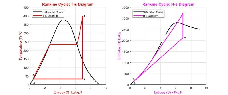
2. Command window showing results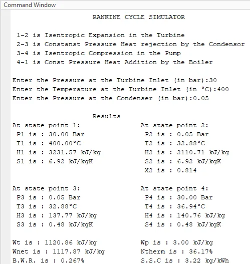
Errors
- At the start encountered few errors for wrong XSteam function. Corrected them by reffering XSteam.m file.
- There was no error in command window but when vapour fraction was showing greater than 1 in few cases (e.g shown in sample output in challange). Highest value of vapour fraction is 1, and because of that enthalpy was calculated incorrect. To correct that used if_else loop for x>=1 & calculated value of enthalpy using Xsteam.
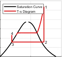
- Initially in T-s diagram, gap was showing in process 4-1 (refer below image). So added an extra point (4a)on saturation curve, divided curve in to parts and plot each section seperately to get continous plot.
References
- https://en.wikipedia.org/wiki/Rankine_cycle#:~:text=The%20Rankine%20cycle%20is%20an,heat%20source%20and%20heat%20sink.
- https://www.hkdivedi.com/2016/09/what-is-rankine-cycle-in-thermal-power.html
- https://www.thermal-engineering.org/what-is-rankine-cycle-steam-turbine-cycle-definition/
- https://www.learnthermo.com/T1-tutorial/ch09/lesson-B/pg07.php
- https://old.amu.ac.in/emp/studym/99995366.pdf
- https://www.nuclear-power.com/nuclear-engineering/materials-nuclear-engineering/properties-steam-what-is-steam/wet-steam/
- https://in.mathworks.com/help/matlab/ref/text.html
- https://in.mathworks.com/matlabcentral/answers/32376-insert-degree-symbol-in-axes-title