Week 3 - Solving second order ODEs

Aim- Write a program in Matlab that solves the ODE of motion of a simple pendulum with damping and simulates the pedulum motion.

The equation of motion of a simple pendulum with damping is as follow-

`(d^2theta)/dt^2+b/m(d theta)/dt+g/Lsin theta=0`

this is an 2nd order ODE. Where b is damping coefficient, g is gravity, L is length of pendulum and m is mass of ball. Initial angular displacement and velocity is 0rad & 3rad/s resp.. Timespan is 0 to 20sec.

To solve this 2nd order equation, first convert it into 1st order ODE, for that let's assume-

`theta=theta1`

`:.(d theta)/dt=(d theta1)/dt=theta2`

`:. (d^2theta)/dt=(d^2theta1)/dt=(d theta2)/dt`

now substituting these values in governing equation, we get-

`(d theta2)/dt+b/mtheta2+g/Lsintheta1=0`

`:.(d theta2)/dt=-b/mtheta2-g/Lsintheta1`

`d/(dt) ((theta1),(theta2))=[[theta2],[-b/mtheta2-g/lsintheta1]]`

To solve this in matlab function is created of inputs od_fun(t, th, b, g, l, m). The code for the same is below-

%% Function to solve 2nd order ODE

function [dth_dt]=od_fun(t,th,b,g,l,m)   % Defining function and variable
% convert 2nd order ODE to 1st order ODE
th1=th(1);
th2=th(2);
dth1_dt=th2;
dth2_dt=-(b/m)*th2-(g/l)*sin(th1);
dth_dt=[dth1_dt;dth2_dt];
end

Main Code-

1. First all the inputs are defined i.e b, g, l, m. Then intial condition and time span is provided in code.
2. to solve 2 1st order ODE used matlab inbuilt ode45 function. in this function, we need to specify 2 inputs (as this is 2nd order so at least inputs are required), ODE function, time span and initial condition.
   
   [t,results]=ode45(@(t,th) od_fun(t,th,b,g,l,m),t_sp,th_0);
3. this result matrix contains 2 columns of which 1st is angular displacement and 2nd is angular velocity w.r.t. time
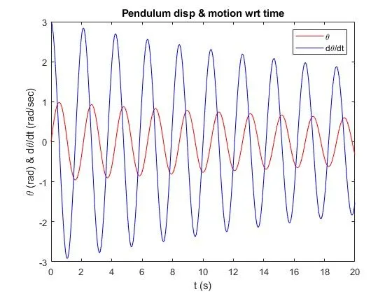
4. using plot commmand this results are plotted wrt time, this plot shows damping effect on pendulum and angular displacement and velocity of pendulum at the specific time. Hold on command is used to plot both graph in same figure(1).
5. For animation of pendulum, we need to show pedulum position at every time interval, to avoid repetative iterations used for loop for length of results(:,1) iterations.
6. One end of pendulum is fixed at (0,0) and other end (x1,y1) are calculated using trignometric relation.
7. all these positiones are retained in figure(2) using hold on command.
8. First fixed line is plotted, then pendulum link is plotted with different linewidth and color. And last pendulum ball is shown using marker command at the end of the link.
9. All these frames are captured as movie frame with getframe(gcf) command.
10. Plot is cleared using hold off command and ct value is increased by 1.
11. An uncompressed Movie file of all captured frames is created using VideoWriter. Then all frame are writen in this video and file is closed.

Final Code-

% Week 3- Solving second order ODEs

clear all
close all
clc

%% Inputs
b=0.05;     % damping coefficient
g=9.81;     % gravity in m/s2
l=1;        % length od pendulum in m
m=1;        % mass of the ball in kg
th_0=[0;3]; % Initial condition
t_sp=linspace(0,20,401);

%% To solve 2nd oreder ODE call function
[t,results]=ode45(@(t,th) od_fun(t,th,b,g,l,m),t_sp,th_0);

%% Plotting
figure(1)
plot(t,results(:,1),'color','r')    % Plot of displacement
hold on                             % Retain plot
plot(t,results(:,2),'color','b')    % Plot of velocity
xlabel('t (s)')
ylabel('\theta (rad) & d\theta/dt (rad/sec)')
legend('\theta','d\theta/dt')
title('Pendulum disp & motion wrt time')

%% Animation
ct=1;
for i=1:length(results(:,1))
    
    % co-ordinates of fixed end
    x0=0;
    y0=0;
    % co-ordinates of moving end of pendulum
    x1=l*sin(results(i,1));
    y1=-l*cos(results(i,1));
    
    %% Plotting for animation
    figure(2)
    % Fixed line plot
    plot([-0.1 0.1], [0 0],'linewidth',5,'color','k')
    hold on         % retain plots
    % Pendulum plot
    plot([x0 x1],[y0 y1],'LineWidth',4,'Color','r')
    % Pendulum Ball
    plot(x1,y1,'o','Markersize',20,'MarkerFaceColor','y','MarkerEdgeColor','k')
    axis([-1 1 -1.2 0.1])   % Frame size
    title('Pendulum Animation','FontSize',14)
    legend('Fixed End','Pendulum link','Ball')
    M(ct)=getframe(gcf);    % Capture fig as movie frame
    hold off                % clear existing plot
    ct=ct+1;                % frame no
end

%% Movie file
movie(M)
% Create file
videofile=VideoWriter('pendulum_animation.avi','Uncompressed AVI');
open(videofile)             % Open the videofile
writeVideo(videofile,M)     % Writing movie M in video file
close(videofile)

Output

1. 
   
2. 
   
   https://youtu.be/zAT8G7XFDOA

Errors

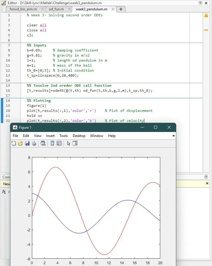
1. When ran 1st half of the program, plot wasn't as expected. Checked all the values, inputs, fuctions everything was right. Then checked the units and standard program in video, found that i used sind(th) instead of sin(th) as angle is in radians.
   
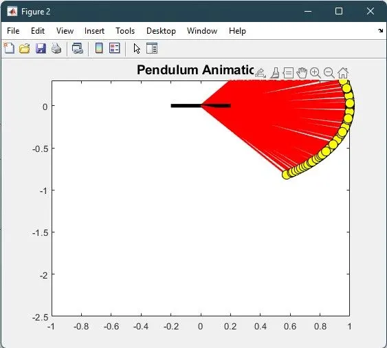
2. The 2nd error was orriention of penndulum in animation (refer image from error 3). it was horizontal. So i interchanged x & y co-ordinates and put '-' sign in y cordinate for correct orientation.
3. 3rd error was all the frames were retained in the animation. I compared it with 2R robotic arm program but no change in output. Then use matlab help and searched for pendulum program and found that instead of pause need to use hold off command to clear the plot.