Code to solve Otto cycle to create PV diagram and find thermal efficiency

Aim- Write code that can solve an otto cycle and make plots for it.

Required output- 1) PV diagram 2) Thermal efficiency

Theory- Otto cycle is used in petroleum based IC engines, where spark plug is used to iginte the fuel, therefore also known as Spark-Ignited(SI) Engines. It has four strokes.

1. Isentropic compression (1-2)- piston moves from BDC to TDC
2. Heat addition at constant volume Qin (2-3)- by ignition of fuel-air mixture
3. Isentropic expansion (3-4)- Power stroke
4. Heat rejection at constant volume Qout (4-1)

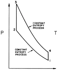
Assume air enter at point 1 is at 300K and 1 atm pressure. And at point 3 temperature is 1330K. Cp and Cv of air is 1.01& 0.718kJ/kg. Engine geometric parameters are bore-0.08m, stroke of cylinder 0.1m coneecting rod length is 0.15 and Compression ratio is 14.

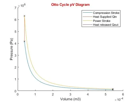
To plot pv diagram, we need 4 state variables- 1 (v1,p1), 2 (v2, p2), 3(v3,p3), 4(v4,p4). From the given input, first we can calculate Swept volume and clearance volume.

Volume of cylinder is, `Vs=pi/4 D^2 L= pi/4 xx text(bore)^2 xx stroke`

and clearance volume is, `Vc=frac{Vs} {(Cr-1)}`

At point 1 & 4 piston is at BDC hence,

`V1=V4=Vs+Vc`

& at point 2 & 3, piston is at TDC hence volume is equal to clearance volume,

`V2=V3=Vc`

Now to find Pressure at every point,

1. Pressure and Temperature at point 2
   Process 1-2 is isentropic compression, hence we can say
   `P1V1^k=P2V2^k=Constant`
   `therefore P2=P1xx(text(V1)/text(V2))^k=P1xx Cr^k`
   T2 can be found using ideal gas equation
   `text(P1V1)/text(T1)=text(P2V2)/text(T2) =text(Constant)`
   `therefore T2=(P2xxV2xxT1)/(P1xxV1)`
2. Pressure at point 3
   T2 can be found using ideal gas equation
   `text(P2V2)/text(T2)=text(P3V3)/text(T3) =text(Constant)`
   `therefore P3=(P2xxT3)/(T2) .. V2=V3 (text(Constant vol process))`
   
3. Pressure at point 4
   `P3V3^k=P4V4^k=text(Constant)`
   `therefore P4=P3xx((V3)/(V4))^k`

Now we can plot all state variables using plot command in matlab. Used figure and hold on command to get all the curves and graph in same figure.

But we cannot join all the points with straight line since process -12 and 3-4 are isentropic compression and expansion resp. So to find volume and pressure at every crank angle we use below formula-

`V/(Vc)=1+1/2(Cr-1)(R+1-Costheta-(R^2-sin^2theta)^(1/2))`

`therefore V=[1+1/2(Cr-1)(R+1-Costheta-(R^2-sin^2theta)^(1/2))]xxVc`

where, R=`R=text(Conn rod length)/a`

and `a=text(crank pin radius)=text(stroke)/2`

for 1-2 isentropic compression process,

`P1V1^k=PcompxxVcomp=text(constant)`

`therefore Pcomp=(P1V1^k)/(Vcomp^k)`

Similarly,

`Pexp=(P3V3^k)/text(Vexp)^k`

from this equation we find pressure and volume in compression and expansion process and plot the curve for pressure and volume for every crank angle.

To avoid repetative use of formula for created a function of(bore, stroke, connecting rod length, compression ratio, start crank angle, end crank angle) to calculate volume. Linspace command is used to get crank angle positions. The code for the same is below-

% Function to calculate volume during compression and expansion stroke
function [v]=otto_cyc_fun(b,s,c,cr,th_s,th_e)

crp=s/2;      % Crank Pin radius
R=c/crp;

% Volume calculation
vs=(pi/4)*b^2*s;        % Swept Volume(Vs)=(pi/4)*Bore^2*stroke
vc=vs/(cr-1);           % Clearance Volume

% Volume inside combustion chamber at different crank position
th=linspace(th_s,th_e,181);
v=(1+0.5*(cr-1)*(R+1-cosd(th)-(R^2-sind(th).^2).^0.5)).*vc;

end

2) Thermal efficiency-

The thermal efficiency is calculated as,

`eta=text(Workdone)/text(Heat supplied)=W/text(Qin)=text(Qin-Qout)/text(Qin)`

`therefore eta=1-text(Qout)/text(Qin)=1-(m.Cv.(T4-T1))/(m.Cv(T3-T2))`

`therefore eta=1-(T4-T1)/(T3-T2)=1-(T1((T4)/(T1)-1))/(T2((T3)/(T2)-1)) .. (i)`

from isentropic equation, `(P1)/(P2)=((V1)/(V2))^k`

and ideal gas eqn, `(P1V1)/(T1)=(P2V2)/(T2)`

`T2=T1(P2V2)/(P1V1)=T1((V1)/(V2))^k((V2)/(V1))=T1Cr^(k-1)`

Similarly, `T3=T4.Cr^(k-1)`

From above equations,

`(T2)/(T1)=(T3)/(T4)=Cr^(k-1)`

`therefore (T3)/(T2)=(T4)/(T1)`

Now in equation of efficiency

`eta=1-(T1)/(T2)=1-(T1)/(T1 Cr^(k-1))=1-1/(Cr^(k-1)`

This is final equation of thermal efficiency

The final code is

% Program for Otto cycle PV diagram and thermal eff
clear all
close all
clc

%% Inputs
p1=101325;  % Pressure at point 1
t1=300;     % Temperature at point 1
t3=1330;    % Temperature at point 3
cp=1.01;    % Sp. heat at constant air pressure
cv=0.718;   % Sp. heat at constant air volume
k=cp/cv;    % sp heat ratio(gamma)=Cp/Cv

% Geometric parameters
b=0.08;     % Bore of cylinder
s=0.1;      % Stroke of cylinder
c=0.15;     % Connecting rod
cr=14;      % Compression ratio

% Volume calculation
vs=(pi/4)*b^2*s;        % Swept Volume(Vs)=(pi/4)*Bore^2*stroke
vc=vs/(cr-1);           % Clearance Volume
v1=vs+vc;               % Volume at point 1 & 4
v2=vc;                  % Volume at point 2 & 3

%% State Variable calculation
% 1-2 is isentropic compression p1v1^k=p2v2^k=constant
p2=p1*cr^k;
% from ideal gas equation p1v1/t1=p2v2/t2
t2=p2*v2*t1/(p1*v1);
% Calling function to calculate compression volume from 180 to 0.
v_comp=otto_cyc_fun(0.08,0.1,0.15,14,180,0);
c_comp=p1*v1^k;
p_comp=c_comp./v_comp.^k;

% 2-3 is heat addition process at constant volume v2=v3
v3=v2;      % Constant Volume process
% from ideal gas equation p2v2/t2=p3v3/t3
p3=p2*t3/t2;

% Process 3-4 is isentropic expansion p3v3^k=p4v4^k
v4=v1;
p4=p3*(v3/v4)^k;
% Calling fun to calculate expanson volume from 0 to 180.
v_exp=otto_cyc_fun(0.08,0.1,0.15,14,0,180);
c_exp=p3*v3^k;
p_exp=c_exp./v_exp.^k;

%% Thermal Efficiency(n)=workdone/Heat supplied=(Qin-Qout)/Qin
% n=1-(Qout/Qin)=1-((T4-T1)/(T3-T2))=1-(1/cr^(k-1))
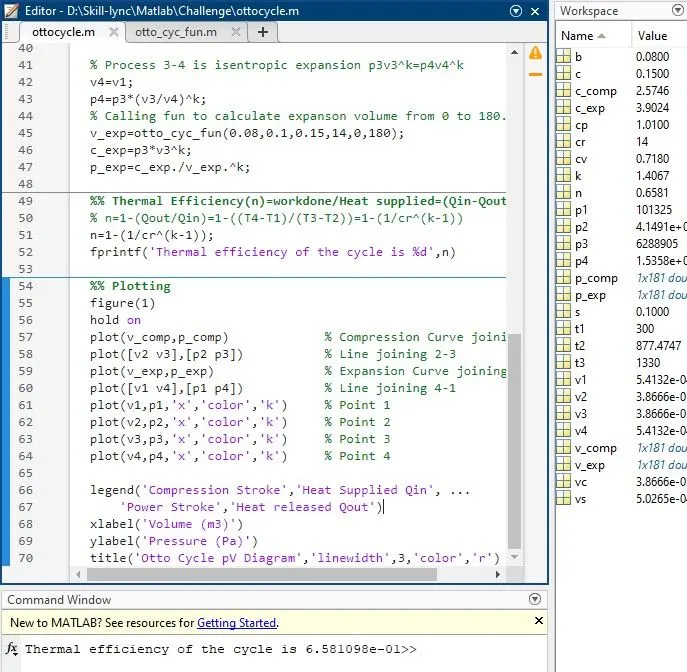
n=1-(1/cr^(k-1));
fprintf('Thermal efficiency of the cycle is %d',n)

%% Plotting
figure(1)
hold on
plot(v_comp,p_comp)             % Compression Curve joining 1-2
plot([v2 v3],[p2 p3])           % Line joining 2-3
plot(v_exp,p_exp)               % Expansion Curve joining 3-4
plot([v1 v4],[p1 p4])           % Line joining 4-1
plot(v1,p1,'x','color','k')     % Point 1 
plot(v2,p2,'x','color','k')     % Point 2
plot(v3,p3,'x','color','k')     % Point 3
plot(v4,p4,'x','color','k')     % Point 4

legend('Compression Stroke','Heat Supplied Qin', ...
    'Power Stroke','Heat released Qout')
xlabel('Volume (m3)')
ylabel('Pressure (Pa)')
title('Otto Cycle pV Diagram','linewidth',3,'color','r')

Output

1. PV diagram

2. Thermal efficiency

We can change compression ration and see its effect on efficiency or we can change other inputs and solve problem. Also Using this method, other air standard cycle problems can be solved.