Week 4.1 - Genetic Algorithm

AIM : To optimise stalagmite function and finding the global maxima of the function by using matlab.

Introduction : Firstly we should know what is optimisation, Optimisation is basically an area to study that deals with how to minimise and maximise the function which depends on multiple input parameters, Because at the end that is going to do. There are several to go about optimisation.

Today we are introducing in to this area

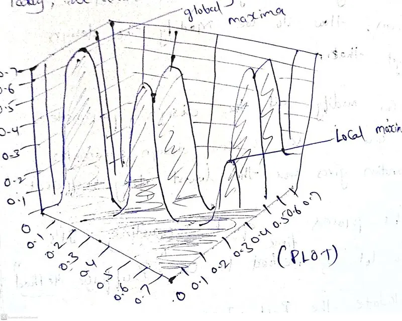
Stalagmite is a actually a mathematically model, This is going to help us to give local minimas and maximas.

Here stalagmite is a formula based function which has already code written in this function. we should call this function when we require in the correct destination.

By using the stalagmite function we can find the global minimas and maximas.

Optimisation is decision making process, It finds to help us the best results under a set of prioritized criteria or constraints.

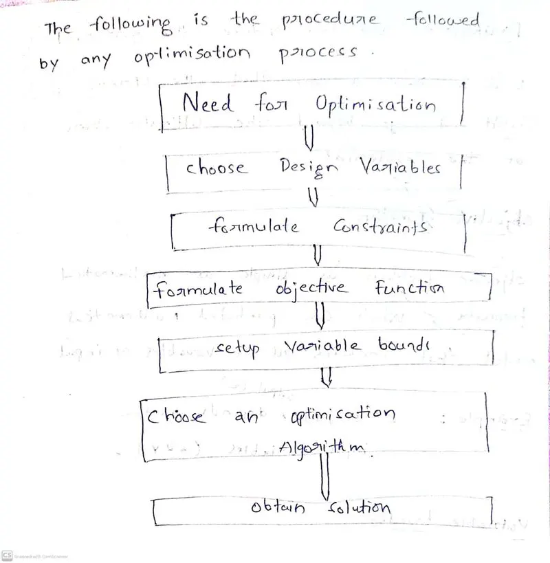
Below is the table for the process of optimisation

GENETIC ALGORITHM (GA) :

As shown in the above table we need to choose an optimisation algorithm to perform optimisation process.

Genetic algorithm is one of the optimisation process.

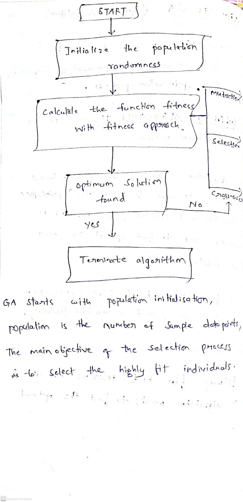
GA is a search based optimisation technique based on the principles of genetics and natural selection. it is frequently used to find optimal or near optimal solutions.

Process for GA

FORMULAS :

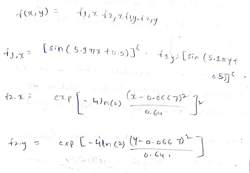
The above formulas are coded in stalagmite function.

PROCEDURE :

Here we are using two variables x and y, Using the linspace command we are creating 150 values between 0 to 0.6.

It is a one dimensional so by using meshgrid we are converting to two dimensional, Assinging the values to inputs by using for loop.

Creating a variable and assinging the number to which the number of iterations performed.

After that solve the stalagmite function using genetic algorithm and assinging to variables.

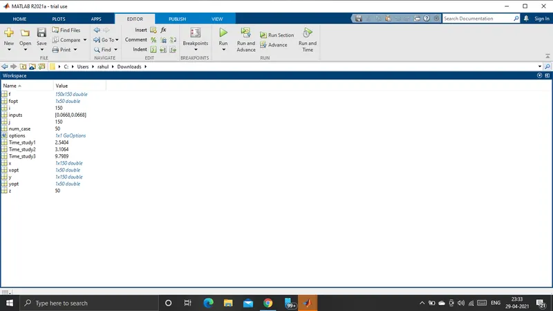
After that we should plot the 3 plots for Bounded inputs, Unbounded inputs, Increased population.

CODE FOR STALAGMITE :

function [f]=stalagmite(V)
x = V(1);
y = V(2);

f1x=(sin((5.1*pi*x)+0.5))^6;
f1y=(sin((5.1*pi*y)+0.5))^6;
f2x=exp(-4*log(2)*(((x-0.0667)^2)/0.64));
f2y=exp(-4*log(2)*(((y-0.0667)^2)/0.64));

f=-(f1x*f1y*f2x*f2y);

CODE FOR GENETIC ALGORITHM :

close all
 clear all
 clc
 % defining the search space
 x = linspace(0,0.6,150);
 y = linspace(0,0.6,150);
 % to create 2d mesh
%   [xx,yy] = meshgrid(x,y);
%  % assigning valus to inputs
  for i = 1:length(x)% takes values until length of xx
      for j = 1:length(y)% takes values until length of xx
          inputs(1) = x(i);
          inputs(2) = y(j);
          f(i,j) = stalagmite(inputs);
      end
  end
 num_case = 50; % creating a variable and assigning the number to which iterations performed
%  f = get_stalagmite(x,y);
 tic % Starts the timer
 % Study case-1
 for z = 1:num_case % takes values until length of num_cases
         [inputs,fopt(z)]  = ga(@stalagmite,2);% solve stalagmite function using GA and assigning to variables
         xopt(z) = inputs(1);
         yopt(z) = inputs(2);
 end
 Time_study1 = toc; % Gives time taken to perform the case

 figure(1)
 subplot(2,1,1) % creates sub-plot in the figure 
 hold on
 surfc(x,y,-f) % Creates a surface
 shading interp % varies the color in each line segment and face by interpolating the colormap index or true color value across the line or face.
 plot3(xopt,yopt,-fopt,'marker','o','markersize',5,'markerfacecolor','r')% plot3 command used to plot in 3 axis
 % marker is used to create a visible points on the plot
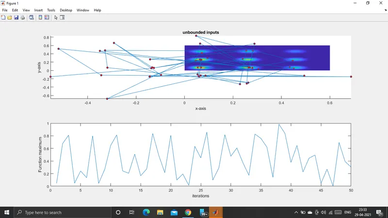
 title('unbounded inputs') 
 xlabel('x-axis')
 ylabel('y-axis')
 zlabel('z-axis')
 subplot(2,1,2)
 plot(-fopt)
 xlabel('iterations')
 ylabel('Function maximum')

% Study Case-2 Defining upper and lower bounds
tic
 for z = 1:num_case
         [inputs,fopt(z)] = ga(@stalagmite,2,[],[],[],[],[0;0],[0.4;0.4]);
         %defines a set of lower and upper bounds on the design variables
         xopt(z) = inputs(1);
         yopt(z) = inputs(2);
 end
 Time_study2 = toc;

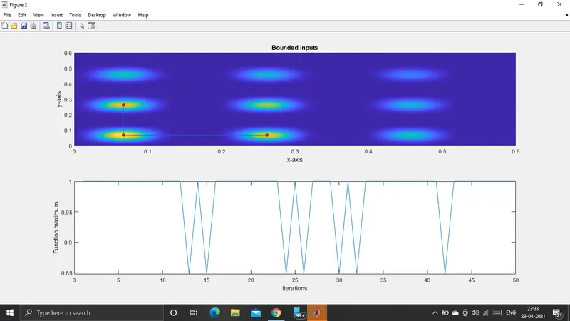
 figure(2)
 subplot(2,1,1)
 hold on
 surfc(x,y,-f)
 shading interp
 plot3(xopt,yopt,-fopt,'marker','o','markersize',5,'markerfacecolor','r')
 title('Bounded inputs')
 xlabel('x-axis')
 ylabel('y-axis')
 zlabel('z-axis')
 subplot(2,1,2)
 plot(-fopt)
 xlabel('iterations')
 ylabel('Function maximum')
 clc
 % Study Case-3 Increasing iterations
 options = optimoptions('ga');% returns a set of default options for the SolverName solver.
 options = optimoptions(options,'PopulationSize',270);%Defining population size
 
 tic
 for z = 1:num_case
         [inputs,fopt(z)]  = ga(@stalagmite, 2,[],[],[],[],[0;0],[0.4;0.4],[],[],options);
         % takes the values of options and solves ga in required population
         xopt(z) = inputs(1);
         yopt(z) = inputs(2);
 end
 Time_study3 = toc;

 figure(3)
 subplot(2,1,1)
 hold on
 surfc(x,y,-f)
 shading interp
 plot3(xopt,yopt,-fopt,'marker','o','markersize',5,'markerfacecolor','r')
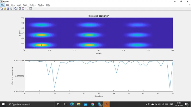
 title('Increased population')
 xlabel('x-axis')
 ylabel('y-axis')
 zlabel('z-axis')
 subplot(2,1,2)
 plot(-fopt)
 xlabel('iterations')
 ylabel('Function maximum')
 % The Global Maximum at the position
%  display(inputs)

OUTPUT :

PLOTS FOR BOUNDED INPUT :

PLOT FOR UNBOUNDED REGION :

PLOT FOR INCREASED POPULATION :

ERRORS :

In this program i found errors like previous challanges in formulas in stalagmite while writing the code and minor errors which was solved later, So i not made any screenshots to show you because i already have a same problem like before while execution of making minor mistakes like putting different logical operators and spelling mistakes.

STEPS TO OVERCOME THOSE ERRORS :

We can resolve those errors by practicing more programs in day to day challanges, We need to take more time while programming for correct execution. I mostly experienced for minor errors takes more time to resolve. 

CONCLUSION :

By this program i have concluded that i optimised the stalagmite function and solved the global maxima of the function.