Week 3.5 - Deriving 4th order approximation of a 2nd order derivative using Taylor Table method
Report on Deriving 4th order approximation of a 2nd order derivative using Taylor Table method
AIM
To derive the following 4th order approximations of the second-order derivative.
1. Central difference
2. Skewed right-sided difference
3. Skewed left-sided difference .After deriving these schemes prove that your skewed schemes are fourth-order accurate
Also to write a program in Matlab to evaluate the second-order derivative of the analytical function exp(x)*cos(x) and compare it with the 3 numerical approximations that are derived.
THEORY
The order of accuracy P = Number of nodes in the stencil N - order of derivative Q + 1 for symmetric/central schemes
The order of accuracy P = Number of nodes in the stencil N - order of derivative Q for one-sided/skewed schemes
Thus number of nodes = P +Q for one-sided/skewed schemes and P+Q-1 for symmetric/central schemes
DERIVATION FOR CENTRAL DIFFERENCE SCHEME:
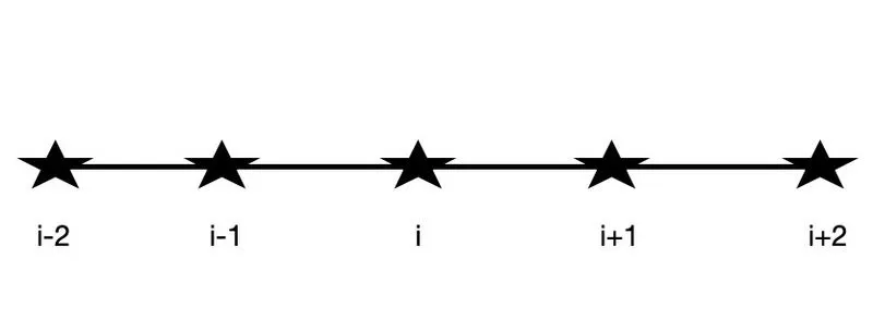
In the central difference scheme we take the number of nodes as 5, because we are asked to derive a 4th order approximations of second order derivative thus we have 4+2-1 = 5 number of nodes, which is taken of the form i-2, i-1, i, i+1, i+2.
We know the hypothesis equation for the 4th order approximation of 2nd order derivative using central difference is
`Deltax^2(del^2f(x))/(delx^2) = af(i-2)+bf(i-1)+cf(i)+df(i+1)+ef(i+2)`
First we take each of the nodes and expand it using Taylor's series, which makes it of the form:
`af(i-2) = a[f(i)-(2Deltaf'(i))/(1!)+((2Deltax)^2f''(i))/(2!)-((2Deltax)^3f'''(i))/(3!)+((2Deltax)^4f''''(i))/(4!)-((2Deltax)^5f'''''(i))/(5!)+((2Deltax)^6f''''''(i))/(6!)]`
`bf(i-1) = b[f(i)-(Deltaxf'(i))/(1!)+((Deltax)^2f''(i))/(2!)-((Deltax)^3f'''(i))/(3!)+((Deltax)^4f''''(i))/(4!)-((Deltax)^5f'''''(i))/(5!)+((Deltax)^6f''''''(i))/(6!)]`
`cf(i) = cf(i)`
`df(i+1) = d[f(i)+(Deltaxf'(i))/(1!)+((Deltax)^2f''(i))/(2!)+((Deltax)^3f'''(i))/(3!)+((Deltax)^4f''''(i))/(4!)+((Deltax)^5f'''''(i))/(5!)+((Deltax)^6f''''''(i))/(6!)]`
`ef(i+2) = e[f(i)+(2Deltaxf'(i))/(1!)+((2Deltax)^2f''(i))/(2!)+((2Deltax)^3f'''(i))/(3!)+((2Deltax)^4f''''(i))/(4!)+((2Deltax)^5f'''''(i))/(5!)+((2Deltax)^6f''''''(i))/(6!)]`
Now using Taylor Table method let us arrange this in a Table which has coefficients in the each rows
| A | f(i) | f'(i)`Deltax` | f''(i)`Deltax^2` | f'''(i)`Deltax^3` | f''''(i)`Deltax^4` | f'''''(i)`Deltax^5` | f''''''(i)`Deltax^6` |
| af(i-2) | a | -2a | 4a/2 | -8a/6 | 16a/24 | -32a/120 | 64a/720 |
| bf(i-1) |
b |
-b | b/2 | -b/6 | b/24 | -b/120 | b/720 |
| cf(i) | c | 0 | 0 | 0 | 0 | 0 | 0 |
| df(i+1) | d | d | d/2 | d/6 | d/24 | d/120 | d/720 |
| ef(i+2) | e | 2e | 4e/2 | 8e/6 | 16e/24 | 32e/120 | 64e/720 |
| `sumA = (del^2f)/(delx^2)` | 0 | 0 | 1 | 0 | 0 | ? | ? |
Here in the first row the coefficient a and its values at each approximation is given at each derivation and at each value of delta x, similarly other rows has the coefficients of the respective nodes and derivatives or in other words Taylor seires terms.
The first column is the hypothesis equation with stencils which is from i-2 to 1+2 is given from row 1 to 5, thus 5 nords are taken and at the last row the sum of all the rows is calculated to calculate the coefficients of the hypothesis equation which is nothing but the second derivative of the function. The values of these summation for each column except the second derivative column will be 0 and the column with the second derivative of the function will be `sumf''(i)Deltax^2 = 1`.
The last two columns of the 5th order and 6th order approximations are given a ? sign because we are not sure whether that value is 0 or not.
The 5 hypothesis equations are:- a+b+c+d+e = 0
-2a-b+0+d+2e = 0
4a/2+b/2+0+d/2+4e/2 = 1
-8a/6-b/6+0+d/6+8e/6 = 0
16a/24+b/24+0+d/24+16e/24 = 0
These equations are converted into matrix form and then the coefficients are calculated
`[[1,1,1,1,1],[-2,-1,0,1,2],[4/2,1/2,0,1/2,4/2],[-8/6,-1/6,0,1/6,8/6],[16/24,1/24,0,1/24,16/24]][[a],[b],[c],[d],[e]] = [[0],[0],[1],[0],[0]]`
Now we have to find the values of coefficients a,b,c,d,e by solving the equations in the matrix
Thus the coefficients will turn out to be
a = -0.0833
b = 1.3333
c = -2.5000
d = 1.3333
e = -0.0833
Let us substitute these coefficients on the equation `Deltax^2(del^2f(x))/(delx^2) = af(i-2)+bf(i-1)+cf(i)+df(i+1)+ef(i+2)`,which turns out to be of the form,
`(del^2f(x))/(delx^2) = (-0.0833f(i-2)+1.3333f(i-1)-2.5000f(i)+1.3333f(i+1)-0.0833f(i+2))/(Deltax^2)`, here we divide the whole term with delta x^2, for calculation purpose.
Now from the taylor table `(del^2f(x))/(delx^2)= (a+b+c+d+e)f(i)+(-2a-b+0+d+2e )f'(i)Deltax+(4a/2+b/2+0+d/2+4e/2 )f''(i)Deltax^2+(-8a/6-b/6+0+d/6+8e/6 )f'''(i)Deltax^3+(16a/24+b/24+0+d/24+16e/24)f''''(i)Deltax^4+(-32a/120-b/120+0+d/120+32e/120)f'''''(i)Deltax^5+(64a/240+b/240+0+d/240+64e/240)f''''''(i)Deltax^6`
In the above equation from the Taylor Table we need the second derivative of the function thus we neglect all other derivatives of functions i.e. (a+b+c+d+e)f(i), (-2a-b+0+d+2e )f'(i)`Deltax`,(-8a/6-b/6+0+d/6+8e/6 )f'''(i) `Deltax^3`,(16a/24+b/24+0+d/24+16e/24)f''''(i)`Deltax^4`are all equal to 0 and also the equation (-32a/120-b/120+0+d/120+32e/120)f'''''(i)`Deltax^5` is also 0 because the sum of the elements/the coefficients is 0
Thus the final equation for forth order approxmation of second order derivative will be :
`Deltax^2(del^2f(x))/(delx^2) =``(4a/2+b/2+0+d/2+4e/2 )f''(i)Deltax^2`+ `(64a/720+b/720+0+d/720+64e/720)f''''''(i)Deltax^6`
After dividing the equation by `Deltax^2`we get the equation as `(del^2f(x))/(delx^2) =(4a/2+b/2+0+d/2+4e/2 )f''(i)`+`(64a/240+b/240+0+d/240+64e/240)f''''''(i)Deltax^4`. In this equation the Delta x^4 is the truncation error and thus makes it the equation for 4th order approximation then we substitute the value a,b,c,d,e in the above equation which makes the equation as
`(del^2f(x))/(delx^2) =((4(-0.0833))/2+1.3333/2+0+1.3333/2+(4(-0.08333))/2 )f''(i)+((64(-0.0833))/720+1.3333/240+0+1.3333/720+(64(-0.0833))/720)f''''''(i)Deltax^4`
DERIVATION FOR SKEWED RIGHT SIDED SCHEME:
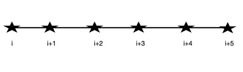
In this scheme we take the number of nodes as per the equation P +Q for one-sided/skewed schemes, thus we have number of nodes = 2+4 = 6. Thus we take the nodes that are of skewed right sided scheme as i,i+1,i+2,i+3,i+4,i+5
The hypothesis equation for the 4th order approximation of 2nd order derivative using skewed right sided difference is
`Deltax^2(del^2f(x))/(delx^2) = af(i)+bf(i+1)+cf(i+2)+df(i+3)+ef(i+4)+gf(i+5)`
First we take each of the nodes and expand it using Taylor's series, which makes it of the form:
af(i) = af(i)
bf(i+1) = `b[f(i)+(Deltaxf'(i))/(1!)+((Deltax)^2f''(i))/(2!)+((Deltax)^3f'''(i))/(3!)+((Deltax)^4f''''(i))/(4!)+((Deltax)^5f'''''(i))/(5!)+((Deltax)^6f''''''(i))/(6!)]`
`cf(i+2) = c[f(i)+(2Deltaxf'(i))/(1!)+((2Deltax)^2f''(i))/(2!)+((2Deltax)^3f'''(i))/(3!)+((2Deltax)^4f''''(i))/(4!)+((2Deltax)^5f'''''(i))/(5!)+((2Deltax)^6f''''''(i))/(6!)]`
`df(i+3) = d[f(i)+(3Deltaxf'(i))/(1!)+((3Deltax)^2f''(i))/(2!)+((3Deltax)^3f'''(i))/(3!)+((3Deltax)^4f''''(i))/(4!)+((3Deltax)^5f'''''(i))/(5!)+((3Deltax)^6f''''''(i))/(6!)]`
`ef(i+4) = e[f(i)+(4Deltaxf'(i))/(1!)+((4Deltax)^2f''(i))/(2!)+((4Deltax)^3f'''(i))/(3!)+((4Deltax)^4f''''(i))/(4!)+((4Deltax)^5f'''''(i))/(5!)+((4Deltax)^6f''''''(i))/(6!)]`
`gf(i+5) = g[f(i)+(5Deltaxf'(i))/(1!)+((5Deltax)^2f''(i))/(2!)+((5Deltax)^3f'''(i))/(3!)+((5Deltax)^4f''''(i))/(4!)+((5Deltax)^5f'''''(i))/(5!)+((5Deltax)^6f''''''(i))/(6!)]`
Now using Taylor Table method let us arrange this in a Table which has coefficients in the each rows
| A | f(i) | f'(i)`Deltax` | f''(i)`Deltax^2` | f'''(i)`Deltax^3` | f''''(i)`Deltax^4` | f'''''(i)`Deltax^5` | f''''''(i)`Deltax^6` |
| af(i) | a | 0 | 0 | 0 | 0 | 0 | 0 |
| bf(i+1) |
b |
b | b/2 | b/6 | b/24 | b/120 | b/720 |
| cf(i+2) | c | 2c | 4c/2 | 8c/6 | 16c/24 | 32c/120 | 64c/720 |
| df(i+3) | d | 3d | 9d/2 | 27d/6 | 81d/24 | 243d/120 | 729d/720 |
| ef(i+4) | e | 4e | 16e/2 | 64e/6 | 256e/24 | 1024e/120 | 4096e/720 |
| gf(i+5) | g | 5g | 25g/2 | 125g/6 | 625g/24 | 3125g/120 | 15625g/720 |
| `sumA = (del^2f)/(delx^2)` | 0 | 0 | 1 | 0 | 0 | 0 | ? |
Here in the first row the coefficient a and its values at each approximation is given at each derivation and at each value of delta x, similarly other rows has the coefficients of the respective nodes and derivatives or in other words Taylor seires terms.
Here also the values of these summation for each column except the second derivative column will be 0 and the column with the second derivative of the function will be `sumf''(i)Deltax^2 = 1`.
The last column of the 6th order approximations are given a ? sign because we are not sure whether that value is 0 or not. Thus it is given as unknown.
The hypothesis equation derived are
a+b+c+d+e+g= 0
0+b+2c+3d+4e+5g = 0
0+b/2+4c/2+9d/2+16e/2+25g/2 = 1
0+b/6+8c/6+27d/6+64e/6+125g/6 = 0
0+b/24+16c/24+81d/24+256e/24+625g/24 = 0
0+b/120+32c/120+243d/120+1024e/120+3125g/120 = 0
These equations are converted into matrix form and then the coefficients are calculated
`[[1,1,1,1,1,1],[0,1,2,3,4,5],[0,1/2,4/2,9/2,16/2,25/2],[0,1/6,8/6,27/6,64/6,125/6],[0,1/24,16/24,81/24,256/24,625/24],[0,1/120,32/120,243/120,1024/120,3125/120]][[a],[b],[c],[d],[e],[g]] = [[0],[0],[1],[0],[0],[0]]`
Now we have to find the values of coefficients a,b,c,d,e and g by solving the equations in the matrix
a = 3.7500
b =-12.8333
c = 17.8333
d = -13.0000
e = 5.0833
g = -0.8333
Let us substitute these coefficients on the equation `Deltax^2(del^2f(x))/(delx^2) = af(i)+bf(i+1)+cf(i+2)+df(i+3)+ef(i+4)+gf(i+5)`,which turns out to be of the form
`(del^2f(x))/(delx^2) = (3.7500f(i)-12.8333f(i+1)+17.8333f(i+2)-13.0000f(i+3)+5.0833f(i+4)-0.8333f(i+5))/(Deltax^2)`, here we divide the whole term with delta x^2, for calculation purpose
Now from the taylor table`(del^2f(x))/(delx^2)=(a+b+c+d+e+g)f(i)+(b+2c+3d+4e+5g)f'(i)Deltax+(b/2+(4c)/2+(9d)/2+(16e)/2+(25g)/2)f''(i)Deltax^2+(b/6+(8c)/6+(27d)/6+(64e)/6+(125g)/6)f'''(i)Deltax^3+(b/24+(16c)/24+(81d)/24+(256e)/24+(625g)/24)f''''(i)Deltax^4+(b/120+(32c)/120+(243d)/120+(1024e)/120+(3125g)/120)f'''''(i)Deltax^5+(b/720+( 64c)/720+(729d)/720+(4096e)/720+(15625g)/720)f''''''(i)Deltax^6`
In the above equation from the Taylor Table we need the second derivative of the function thus we neglect all other derivatives of functions i.e (a+b+c+d+e+g)f(i),
`(b+2c+3d+4e+5g)f'(i)Deltax,`(b/6+(8c)/6+(27d)/6+(64e)/6+(125g)/6)f'''(i)Deltax^3, (b/24+(16c)/24+(81d)/24+(256e)/24+(625g)/24)f''''(i)Deltax^4, (b/120+(32c)/120+(243d)/120+(1024e)/120+(3125g)/120)f'''''(i)Deltax^5` are all equal to 0.
Thus the final equation for forth order approxmation of second order derivative will be :
`Deltax^2(del^2f(x))/(delx^2) = (b/2+(4c)/2+(9d)/2+(16e)/2+(25g)/2)f''(i)Deltax^2+(b/720+( 64c)/720+(729d)/720+(4096e)/720+(15625g)/720)f''''''(i)Deltax^6`
After dividing by `Deltax^2` and substituting the values of a,b,c,d,e,and g we have,
`(del^2f(x))/(delx^2) = (-12.8333/2+(4(17.8333))/2+(9(-13.0000))/2+(16(5.0833))/2+(25(-0.8333))/2)f''(i)+((-12.8333)/720+( 64(17.8333))/720+(729(-13.0000))/720+(4096(5.0833))/720+(15625(-0.8333))/720)f''''''(i)Deltax^4`
In this equation the Delta x^4 is the truncation error and thus makes it the equation for 4th order approximation.
DERIVATION FOR SKEWED LEFT SIDED SCHEME:
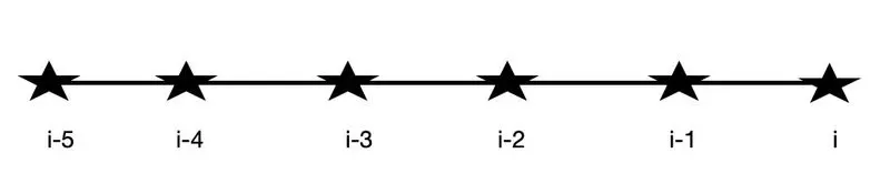
In this scheme again we take the number of nodes as per the equation P +Q for one-sided/skewed schemes, thus we have number of nodes = 2+4 = 6. Thus we take the nodes that are of skewed left sided scheme as i-5,i-4,i-3,i-2,i-1,i i.e the nodes to the left side of i.
The hypothesis equation for the 4th order approximation of 2nd order derivative using skewed right sided difference is
`Deltax^2(del^2f(x))/(delx^2) = af(i-5)+bf(i-4)+cf(i-3)+df(i-2)+ef(i-1)+gf(i)`
Here also we take each of the nodes and expand it using Taylor's series, which makes it of the form:
`af(i-5) = a[f(i)-(5Deltaxf'(i))/(1!)+((5Deltax)^2f''(i))/(2!)-((5Deltax)^3f'''(i))/(3!)+((5Deltax)^4f''''(i))/(4!)-((5Deltax)^5f'''''(i))/(5!)+((5Deltax)^6f''''''(i))/(6!)]`
`bf(i-4) = b[f(i)-(4Deltaxf'(i))/(1!)+((4Deltax)^2f''(i))/(2!)-((4Deltax)^3f'''(i))/(3!)+((4Deltax)^4f''''(i))/(4!)-((4Deltax)^5f'''''(i))/(5!)+((4Deltax)^6f''''''(i))/(6!)]`
`cf(i-3) = c[f(i)-(3Deltaxf'(i))/(1!)+((3Deltax)^2f''(i))/(2!)-((3Deltax)^3f'''(i))/(3!)+((3Deltax)^4f''''(i))/(4!)-((3Deltax)^5f'''''(i))/(5!)+((3Deltax)^6f''''''(i))/(6!)]`
`df(i-2) = d[f(i)-(2Deltaxf'(i))/(1!)+((2Deltax)^2f''(i))/(2!)-((2Deltax)^3f'''(i))/(3!)+((2Deltax)^4f''''(i))/(4!)-((2Deltax)^5f'''''(i))/(5!)+((2Deltax)^6f''''''(i))/(6!)]`
`ef(i-1) = e[f(i)-(Deltaxf'(i))/(1!)+((Deltax)^2f''(i))/(2!)-((Deltax)^3f'''(i))/(3!)+((Deltax)^4f''''(i))/(4!)-((Deltax)^5f'''''(i))/(5!)+((Deltax)^6f''''''(i))/(6!)]`
gf(i) = gf(i)
Now using Taylor Table method let us arrange this in a Table which has coefficients in the each rows
| A | f(i) | f'(i)`Deltax` | f''(i)`Deltax^2` | f'''(i)`Deltax^3` | f''''(i)`Deltax^4` | f'''''(i)`Deltax^5` | f''''''(i)`Deltax^6` |
| af(i-5) | a | -5a | 25a/2 | -125a/6 | 625a/24 | -3125a/120 | 15625a/720 |
| bf(i-4) |
b |
-4b | 16b/2 | -64b/6 | 256b/24 | -1024b/120 | 4096b/720 |
| cf(i-3) | c | -3c | 9c/2 | 27c/6 | 81c/24 | -243c/120 | 729c/720 |
| df(i-2) | d | -2d | 4d/2 | -8d/6 | 16d/24 | -32d/120 | 64d/720 |
| ef(i-1) | e | -e | e/2 | -e/6 | e/24 | -e/120 | e/720 |
| gf(i) | g | 0 | 0 | 0 | 0 | 0 | 0 |
| `sumA = (del^2f)/(delx^2)` | 0 | 0 | 1 | 0 | 0 | 0 | ? |
Here also the values of these summation for each column except the second derivative column will be 0 and the column with the second derivative of the function will be `sumf''(i)Deltax^2 = 1`
The hypothesis equation derived are
a+b+c+d+e+g= 0
-5a-4b-3c-2d-e+0 = 0
25a/2+16b/2+9c/2+4d/2+e/2+0 = 1
-125g/6-64b/6-27c/6-8d/6-e/6+0 = 0
625a/24+256b/24+81c/24+16d/24+e/24+0 = 0
-3125a/120-1024b/120-243c/120-32d/120-e/120+0 = 0
These equations are converted into matrix form and then the coefficients are calculated
`[[1,1,1,1,1,1],[-5,-4,-3,-2,-1,0],[25/2,16/2,9/2,4/2,1/2,0],[-125/6,-64/6,-27/6,-8/6,-1/6,0],[625/24,256/24,81/24,16/24,1/24,0],[-3125/120,-1024/120,-243/120,-32/120,-1/120,0]][[a],[b],[c],[d],[e],[g]] = [[0],[0],[1],[0],[0],[0]]`
a = -0.8333
b =5.0833
c = -13.0000
d = 17.8333
e = -12.8333
g = 3.7500
Let us substitute these coefficients on the equation `Deltax^2(del^2f(x))/(delx^2) = af(i-5)+bf(i-4)+cf(i-3)+df(i-2)+ef(i-1)+gf(i)`which turns out to be of the form
`(del^2f(x))/(delx^2) =(-0.8333f(i-5)+5.0833f(i-4)+(-13.000)f(i-3)+17.8333f(i-2)+(-12.8333)f(i-1)+3.7500f(i) )/(Deltax^2)`,` here we divide the whole term with delta x^2, for calculation purpose
Now from the taylor table, `(del^2f(x))/(delx^2)=(a+b+c+d+e+g)f(i)+(-5a-4b-3c-2d-e+0)f'(i)Deltax+((25a)/2+(16b)/2+(9c)/2+(4d)/2+(e)/2+0)f''(i)Deltax^2+((-125a)/6+(-64b)/6+(-27c)/6+(-8d)/6+(-e)/6+0)f'''(i)Deltax^3+((625a)/24+(256b)/24+(81c)/24+(16d)/24+(e)/24+0)f''''(i)Deltax^4+((-3125a)/120+(-1024b)/120+(-243c)/120+(-32d)/120+(-e)/120+0)f'''''(i)Deltax^5+((15625a)/720+(4096b)/720+(729c)/720+(64d)/720+(e)/720+0)f''''''(i)Deltax^6`
In the above equation from the Taylor Table we need the second derivative of the function thus we neglect all other derivatives of functions
`(a+b+c+d+e+g)f(i), (-5a-4b-3c-2d-e+0)f'(i)Deltax, ((-125a)/6+(-64b)/6+(-27c)/6+(-8d)/6+(-e)/6+0)f'''(i)Deltax^3, ((625a)/24+(256b)/24+(81c)/24+(16d)/24+(e)/24+0)f''''(i)Deltax^4, ((-3125a)/120+(-1024b)/120+(-243c)/120+(-32d)/120+(-e)/120+0)f'''''(i)Deltax^5` all are equal to zero whereas the second order approximation of the function will be equal to 1 i.e. `sumf''(i)Deltax^2 = 1`.
Thus the final equation for forth order approxmation of second order derivative will be :
((25a)/2+(16b)/2+(9c)/2+(4d)/2+(e)/2+0)f''(i)Deltax^2+((15625a)/720+(4096b)/720+(729c)/720+(64d)/720+(e)/720+0)f''''''(i)Deltax^6`
After dividing by `Deltax^2` and substituting the values of a,b,c,d,e,and g we have,
`(del^2f(x))/(delx^2) = ((25(-0.8333))/2+(16(5.0833))/2+(9(-13.0000))/2+(4(17.8333))/2+(-12.8333)/2+0)f''(i)+((15625(-0.8333))/720+(4096(5.0833))/720+(729(-13.0000))/720+(64(17.8333))/720+(-12.8333)/720+0)f''''''(i)Deltax^4`
In this equation the Delta x^4 is the truncation error and thus makes it the equation for 4th order approximation.
PROGRAM AND ITS DEFINITION
At first we have to define the functions that are used to find the errors for central,skewed right and skewed left sided difference approximations
Function for central difference
function out  = central_difference_scheme(x,dx)

%analytical function exp(x)*cosx
%analytical derivative
%f''(x) = -2*exp(x)*sinx
%af(i-2)+bf(i-1)+cf(i)+df(i+1)+ef(i+2)
a = -1/12
b = 4/3
c = -5/2
d = 4/3
e = -1/12

analytical_derivative = -2*exp(x)*sin(x)

central_differencing = ((a*exp(x-(2.*dx))*cos(x-(2.*dx))+b*exp(x-dx)*cos(x-dx)+c*exp(x)*cos(x)+d*exp(x+dx)*cos(x+dx)+e*exp(x+(2.*dx))*cos(x+(2.*dx))))./(dx.^2);

out = abs(analytical_derivative-central_differencing)
end
In the above function we define the central difference scheme with input values x and dx. Here we know that the analytical derivative(i.e second derivative) of the function is -2*exp(x)*sin(x)
Then we find the central difference scheme by substituting the function in the equation af(i-2)+bf(i-1)+cf(i)+df(i+1)+ef(i+2) which results in the equation
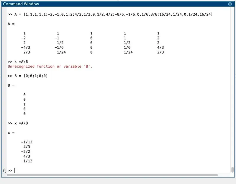
Then we find the error which is here called as 'out' which is, out = abs(analytical_derivative-central_differencing)
Then we end the function using end command
The function for skewed right sided difference
function out  = skewed_right_sided(x,dx)


%analytical function exp(x)*cosx
%analytical derivative
%f''(x) = -2*exp(x)*sinx
%equation = af(i)+bf(i+1)+cf(i+2)+df(i+3)+ef(i+4)+gf(i+5)
a = 15/4
b = -77/6;
c = 107/6;
d = -13;
e = 61/12;
g = -5/6;
analytical_derivative = -2*exp(x)*sin(x)

skewed_right_differencing = ((a*exp(x)*cos(x)+b*exp(x+dx)*cos(x+dx)+c*exp(x+(2*dx))*cos(x+(2*dx))+d*exp(x+(3*dx))*cos(x+(3*dx))+e*exp(x+(4*dx))*cos(x+(4*dx))+g*exp(x+(5*dx))*cos(x+(5*dx))))/(dx^2)

out = abs(analytical_derivative-skewed_right_differencing)
end
Here also the inputs are same only difference is we give the function name skewed_right_sided and we find the skewed right sided difference scheme by substituting the function in the equation af(i)+bf(i+1)+cf(i+2)+df(i+3)+ef(i+4)+gf(i+5) which results in the equation of skewed right sided differencing scheme.
Here we input the values of a,b,c,d,e and g with the values which we solved using matrix inversion technique
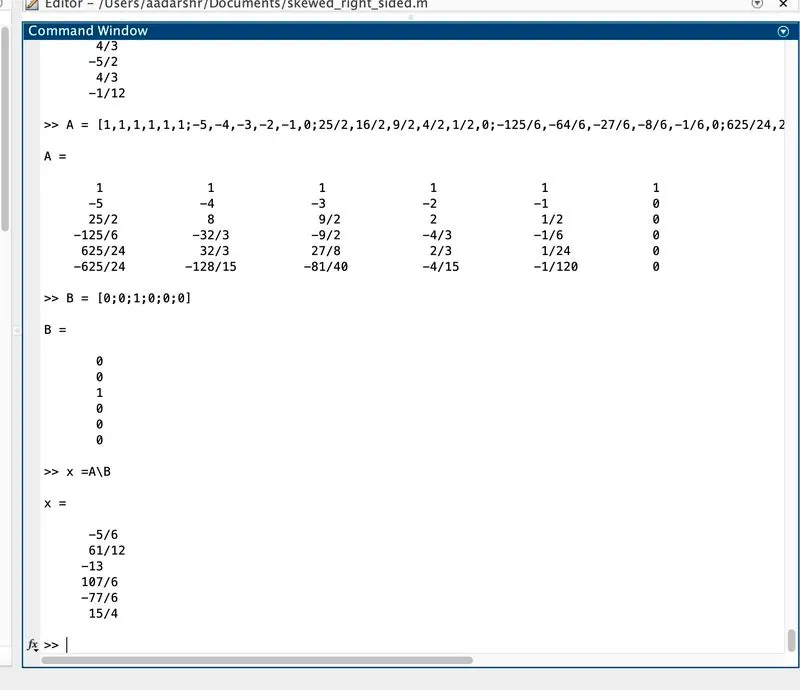
Then we find the error which is here called as 'out' which is, out = abs(analytical_derivative-skewed_right_differencing)
Then we end the function using end command
The function for skewed left sided difference
function out  = skewed_left_sided(x,dx)


%analytical function exp(x)*cosx
%analytical derivative
%f''(x) = -2*exp(x)*sinx
%equation = af(i-5)+bf(i-4)+cf(i-3)+df(i-2)+ef(i-1)+gf(i)
a = -5/6;
b = 61/12;
c = -13;
d = 107/6;
e = -77/6;
g = 15/4;
analytical_derivative = -2*exp(x)*sin(x)

skewed_left_differencing = ((a*exp(x-(5.*dx))*cos(x-(5.*dx))+b*exp(x-(4.*dx))*cos(x-(4.*dx))+c*exp(x-(3.*dx))*cos(x-(3.*dx))+d*exp(x-(2.*dx))*cos(x-(2.*dx))+e*exp(x-dx)*cos(x-dx)+g*exp(x)*cos(x)))./(dx.^2)

out = abs(analytical_derivative-skewed_left_differencing)
end
we find the skewed left sided difference scheme by substituting the function in the equation af(i-5)+bf(i-4)+cf(i-3)+df(i-2)+ef(i-1)+gf(i) which results in the equation of skewed left sided differencing scheme.
Then we find the error which is here called as 'out' which is, out = abs(analytical_derivative-skewed_left_differencing)
Then we end the function using end command
clear all
close all
clc

x = pi/3;
analytical_derivative = -2*exp(x)*sin(x);

% numerical derivative
dx = linspace(pi/4000,pi/4,10);
for i = 1:length(dx)

%central difference approximation
central_difference_error(i) = central_difference_scheme(x,dx(i))

%skewed right sided approximation
skewed_right_error(i) = skewed_right_sided(x,dx(i))

% skewed left sided approximation
skewed_left_error(i) = skewed_left_sided(x,dx(i))
end
loglog(dx,central_difference_error,'color','r','linewidth',3)
hold on
loglog(dx,skewed_right_error,'color','b','linewidth',3)
loglog(dx,skewed_left_error,'color','y','linewidth',3)
xlabel('dx')
ylabel('Absolute error')
legend('central difference','skewed right sided','skewed left sided')- In the above program first we input the input values i.e. x = pi/3 and dx = linspace(pi/4000,pi/4,10), here dx is an array with 10 input values using linspace command, thus we use a for loop which varies from 1:length(dx).
- Inside this loop we call our functions, the calling is carried out for each of the dx values thus while calling we use (i). The calling of the central_difference_scheme, skewed_right_sided and skewed_left_sided functions are done in the same manner i.e. value for each dx is calculated.
central_difference_error(i) = central_difference_scheme(x,dx(i))skewed_right_error(i) = skewed_right_sided(x,dx(i))skewed_left_error(i) = skewed_left_sided(x,dx(i))
- Then we end the loop using end command
- Next step is to plot the error against dx, for that here we use loglog. command rather than plot command because loglog command is used when two plots are having large difference in magnitude and the plotting of such values using normal plot command will be difficult to understand thus we need to use log command. Here we use loglog as the command because we have two input values.
- Then we label the x axis and yaxis as dx and 'Absolute error' and also provide the legend command to distinguish the plot.
clear all
close all
clc

x = pi/3;
analytical_derivative = -2*exp(x)*sin(x);

% numerical derivative
dx = linspace(pi/4000,pi/4,10);
for i = 1:length(dx)

%central difference approximation
central_difference_error(i) = central_difference_scheme(x,dx(i))

%skewed right sided approximation
skewed_right_error(i) = skewed_right_sided(x,dx(i))

% skewed left sided approximation
skewed_left_error(i) = skewed_left_sided(x,dx(i))
end
loglog(dx,central_difference_error,'color','r','linewidth',3)
hold on
loglog(dx,skewed_right_error,'color','b','linewidth',3)
loglog(dx,skewed_left_error,'color','y','linewidth',3)
xlabel('dx')
ylabel('Absolute error')
legend('central difference','skewed right sided','skewed left sided')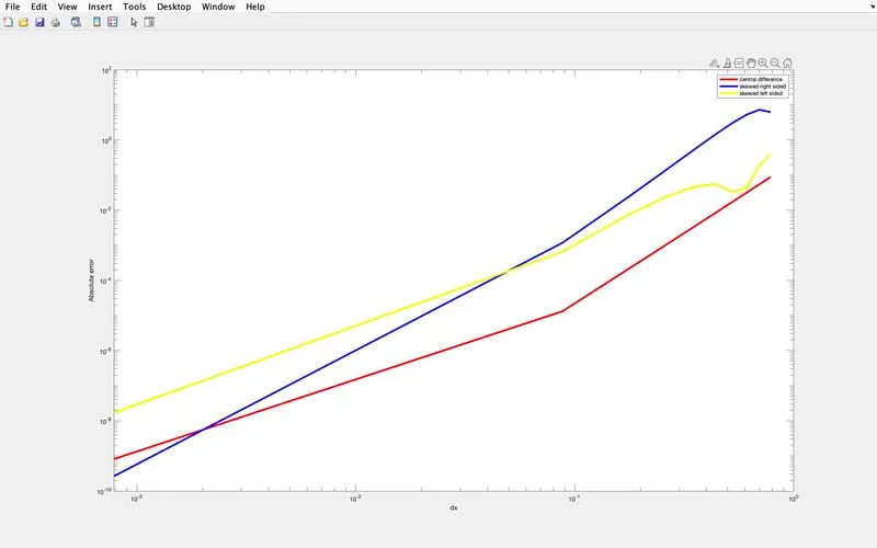
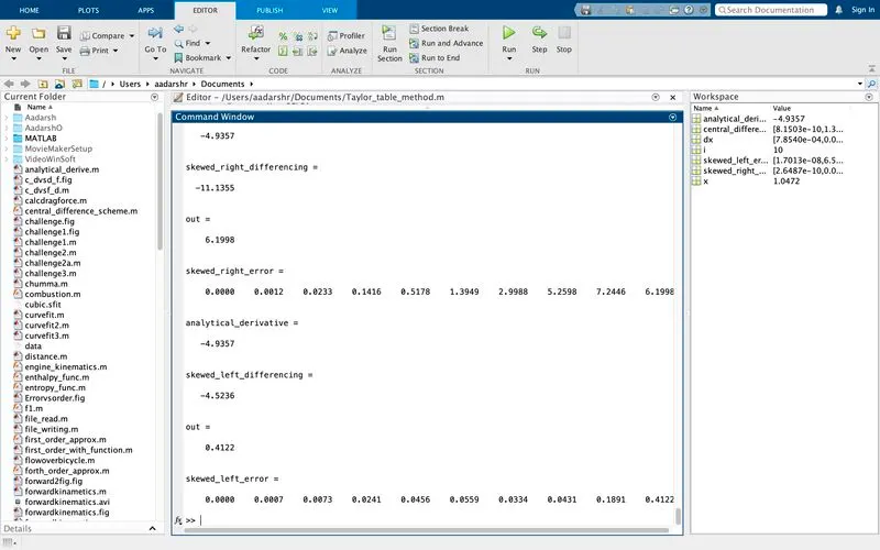
when dx = linspace(pi/400,pi/4,10)
clear all
close all
clc

x = pi/3;
analytical_derivative = -2*exp(x)*sin(x);

% numerical derivative
dx = linspace(pi/400,pi/4,10);
for i = 1:length(dx)

%central difference approximation
central_difference_error(i) = central_difference_scheme(x,dx(i))

%skewed right sided approximation
skewed_right_error(i) = skewed_right_sided(x,dx(i))

% skewed left sided approximation
skewed_left_error(i) = skewed_left_sided(x,dx(i))
end
loglog(dx,central_difference_error,'color','r','linewidth',3)
hold on
loglog(dx,skewed_right_error,'color','b','linewidth',3)
loglog(dx,skewed_left_error,'color','y','linewidth',3)
xlabel('dx')
ylabel('Absolute error')
legend('central difference','skewed right sided','skewed left sided')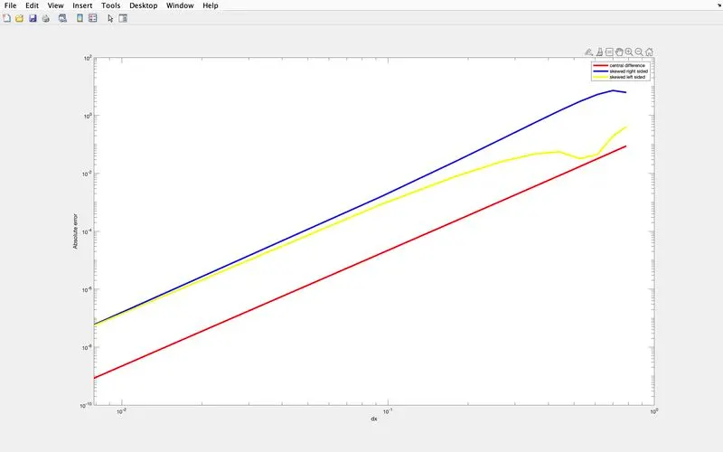
From the above plot we can conclude that cemtral difference scheme has lesser error with decreasing dx as compared to the skewed right sided and skewed left sided schemes.
RESULT
The 4th order approximations of the second-order derivative of Central difference , Skewed right-sided difference, Skewed left-sided difference and the program in Matlab to evaluate the second-order derivative of the analytical function exp(x)*cos(x) and compare it with the 3 numerical approximations that are derived are successfully completed.
Here we have been asked 2 questions:
1.why a skewed scheme is useful?
Skewed scheme is useful when there aren't sufficient information available, in such cases the numerical stencil might not be symmetric. Thus we use skewed scheme.
2.What can a skewed scheme do that a CD scheme cannot?
Since there are no boundaries or sufficient information available CD scheme cannot be used to find the value at the specified point thus we use skewed scheme in place of CD scheme even though CD scheme is more accurate than the skewed scheme and has lesser error as compared to skewed scheme.
CONCLUSION
From the above plot we can conclude that cemtral difference scheme has lesser error with decreasing dx as compared to the skewed right sided and skewed left sided schemes and the 4th order approximations of the second-order derivative of Central difference , Skewed right-sided difference, Skewed left-sided difference and the program in Matlab to evaluate the second-order derivative of the analytical function exp(x)*cos(x) and compare it with the 3 numerical approximations that are derived are successfully completed.