Week 4.1 - Genetic Algorithm

GENETIC ALGORITHM - The genetic algorithm is a method for solving both constrained and unconstrained optimization problems that is based on natural selection, the process that drives biological evolution. The genetic algorithm repeatedly modifies a population of individual solutions. At each step, the genetic algorithm selects individuals from the current population to be parents and uses them to produce the children for the next generation. Over successive generations, the population "evolves" toward an optimal solution. You can apply the genetic algorithm to solve a variety of optimization problems that are not well suited for standard optimization algorithms, including problems in which the objective function is discontinuous, nondifferentiable, stochastic, or highly nonlinear. The genetic algorithm can address problems of mixed integer programming, where some components are restricted to be integer-valued.

SELECTION RULES - The genetic algorithm uses three main types of rules at each step to create the next generation from the current population: Selection rules select the individuals, called parents, that contribute to the population at the next generation. The selection is generally stochastic, and can depend on the individuals' scores.

CROSSOVER RULES - Crossover is the most significant phase in a genetic algorithm. For each pair of parents to be mated, a crossover point is chosen at random from within the genes.

MUTATION RULES - Mutation is a genetic operator used to maintain genetic diversity from one generation of a population of genetic algorithm chromosomes to the next. It is analogous to biological mutation.

OPTIMIZATION -

Optimization refers to finding the values of inputs in such a way that we get the “best” output values. The definition of “best” varies from problem to problem, but in mathematical terms, it refers to maximizing or minimizing one or more objective functions, by varying the input parameters.

The set of all possible solutions or values which the inputs can take make up the search space. In this search space, lies a point or a set of points which gives the optimal solution. The aim of optimization is to find that point or set of points in the search space.

ECONOMIES - It has been used to characterize a variety of models including the cobweb model, the overlapping generations model, game theory, schedule optimization and asset pricing.

NEURAL NETWORKS - a neural network consists of a series of algorithms that endeavor to determine and identify patterns. It works similarly to how a human brain’s neural network works. In algorithms, a neural network refers to a network of neurons, where a neuron is a mathematical function used to collect as well as to classify data from a given model.

IMAGE PROCESSING - Genetic Algorithms (GAs) are increasingly being explored in many areas of image analysis to solve complex optimization problems.

FITNESS FUNCTION - The fitness function simply defined is a function which takes a candidate solution to the problem as input and produces as output how “fit” our how “good” the solution is with respect to the problem in consideration.

THE SYNTAX OF GA IN MATLAB

x=ga(fun,nvars,A,B,Aeq,Beq,,lb,ub,nonlcon,intcon,options)

• 'x' variable to store the output of the genetic algorithm.
• 'fun' to call the function.
• 'A' nad 'B' are used to represent the linear inequalities of the function,if the linear inequalities do not exist they can be set as empty[].
• 'lb'and 'ub' are used to specify the upper and lower bounds of the variable of the function.
• 'nonclon'represents the integers constraints ,such that the value of trhe function is an integer.
• 'options' used to provide the value of the default parameter ,if it is required to replace the parameter .this is done by using the 'optimoptions'.

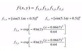
STALAGMITE FUNCTION - It creates local maxima and local minimas for data and also helps in finding best design characteristics for a product. And to solve the Stalagmite function we need Genetic Algorithms as it gives us the global mimas for the data and even for a parameter declared.

FUNCTION PROGRAM

function[f]=stalagmite(input_vector)


a=input_vector(1);
b=input_vector(2);
f1_x=[sin((5.1*pi*a)+0.5)].^6;
f1_y=[sin((5.1*pi*b)+0.5)].^6;
f2_x=exp(-4*log(2)*(((a-0.0667)^2)/(0.64)));
f2_y=exp(-4*log(2)*(((b-0.0667)^2)/(0.64)));

f=-(f1_x*f1_y*f2_x*f2_y);
end

Negative command is used to invert the plot as the ga command find only minimum point.

MAIN PROGRAM

clear all 
close all
clc
x=linspace(0,0.6,150);
y=linspace(0,0.6,150);
[xx , yy]=meshgrid(x,y);

for i=1:length(xx)
    for j=1:length(yy)
    input_vector(1)=xx(i,j);
    input_vector(2)=yy(i,j);
    f(i,j)=stalagmite(input_vector);
    end

end
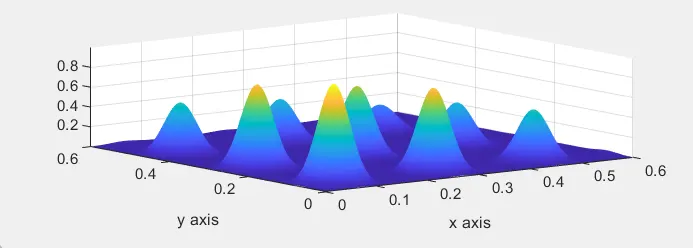
surfc(xx,yy,-f)
shading interp
[inputs,fval]=ga(@stalagmite,2);
xlabel('x axis')
ylabel('y axis')

• Clear all,close all,clc clear the all command window.
• x and y values using the linspace command .if we set lower and upper limits and number of values need it takes random values.
• meshgrid command is used in order to form an array of row and column and it stored in xx and yy .
• we call the stalagmite function (input_vector).
• surfc command is used to get a plot as a surface.
• shading interp command is used to remove the grid structure on the plot .
• ga command is used to, call the the stalagmite function we enter the number of variable .we have two variable x and y.
• x label and y label is used to get a plot clearly.

MAIN PROGRAM PLOT

STUDY- 1 STASTISTICAL BEHAVIOR PROGRAM

%study-1 stastistical behavior
num_cases=50

tic
for i=1:num_cases
    [inputs1,fopt1(i)]=ga(@stalagmite,2);
    xopt1(i)=inputs1(1);
    yopt1(i)=inputs1(2);
end
study1_time=toc;
mean1=-(mean(fopt1));

figure(1)
subplot(2,1,1)

surfc(x,y,-f)
shading interp
hold on
plot3(xopt1,yopt1,-fopt1,'marker','o','markersize',5,'MarkerFaceColor','r');
title('unbounded inputs')
xlabel('x-axis')
ylabel('y-axis')
subplot(2,1,2)
plot(-fopt1)
xlabel('Iterations')
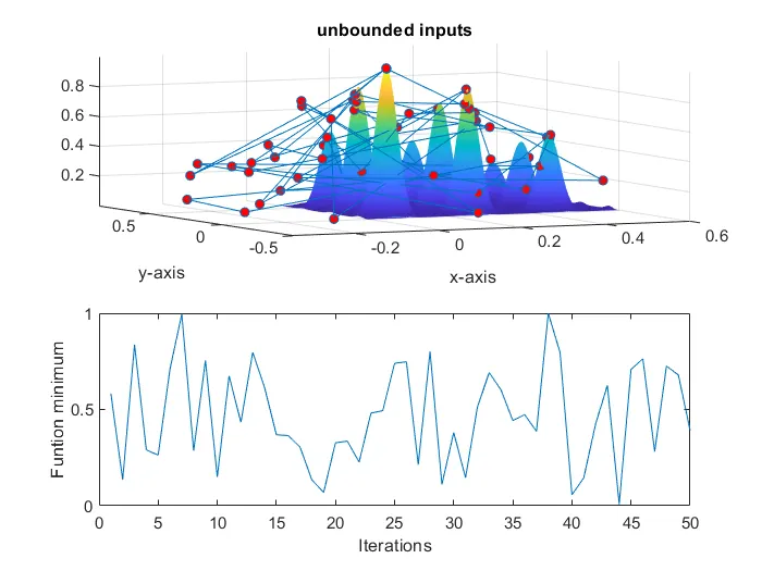
ylabel('Funtion minimum')

• In this study ,we introduce the number num_cases=50 in this program. the 50 indicates that 50 times the ga need to repeat and it calculates the value.
• the tic command is used in order to find out the time taken .
• for loop command is used length of its sets as the number of cases.
• ga command is used as before calling the function and the number variable in the program.
• the calculated x and y values are stored in xopt1 and yopt 1 .
• subplot command is used to in order to grt number of plots in the same single figure plot.
• in the first plot x,y,f as a surface by using the surface command.
• the negative sign is used in the function (f) plotting we invert and we need to rever it back .
• plot calculated maximum value as a dot structure by using the marker and marker size.
• for thr title used the title command.
• subplot command is used to same figure window.
• valus and the number of iterations the xlabel and ylabel is mentioned.
• in the studt we get a random value and we did not get an exact global maxima value .

STUDY-2 STASTISTICAL BEHAVIOR WITH UPPER AND LOWER BOUND LIMITS: PROGRAM

%study-2 statistical behavior with upper and lower bound limits

     
tic
for i=1:num_cases
    [inputs2,fopt2(i)]=ga(@stalagmite,2,[],[],[],[],[0,0],[1,1]);
    xopt2(i)=inputs2(1);
    yopt2(i)=inputs2(2);
end
study2_time=toc;
mean2=-(mean(fopt2));

figure(2)
subplot(2,1,1)

surfc(x,y,-f)
shading interp
hold on
plot3(xopt2,yopt2,-fopt2,'marker','o','markersize',5,'MarkerFaceColor','r');
title('unbounded inputs')
xlabel('x-axis')
ylabel('y-axis')
subplot(2,1,2)
plot(-fopt2)
xlabel('Iterations')
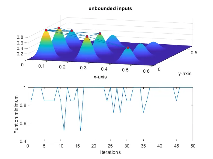
ylabel('Funtion mini

• From the previous study ,we inferred that the search space of the ga is not within the search space so to overcome this error we used the bounded script method.
• as the name suggest in this study we will enter the boundary and within the boundary ,only the ga perform.
• all the command used in the study are also the same in the previous study.
• in this study as mentioned above the limit criteria ,we call the stalagmite,function and the number of variable mentioned as done earlier and we enter the lower and upper boundary limits value.
• in our program ,the lower boundary limit is set as 0,0 and the upeer limit 1,1.
• this is study is better than previous study .

STUDY-3 INCREASING GA ITERATIONS PROGRAM

%study-3 increasing GA iterations

options=optimoptions('ga')
options=optimoptions(options,'populationsize',400);



tic
for i=1:num_cases
    [inputs3,fopt3(i)]=ga(@stalagmite,2,[],[],[],[],[0,0],[1,1],[],[],options);
    xopt3(i)=inputs3(1);
    yopt3(i)=inputs3(2);
end
study3_time=toc;
mean3=-(mean(fopt3));

figure(3)
subplot(2,1,1)

surfc(x,y,-f)
shading interp
hold on
plot3(xopt3,yopt3,-fopt3,'marker','o','markersize',5,'MarkerFaceColor','r');
title('Bounded inputs with modified population size')
xlabel('x-axis')
ylabel('y-axis')
subplot(2,1,2)
plot(-fopt3)
xlabel('Iterations')
ylabel('Funtion minimum')

• All the command is used in the previus study.
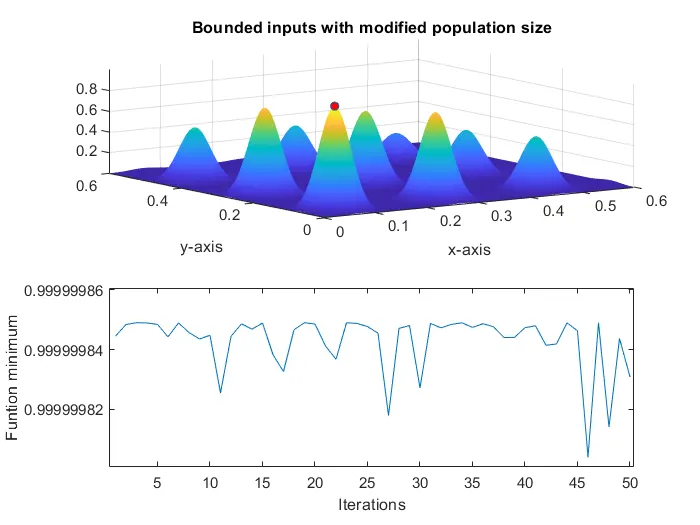
• in this optimization technique is used to set the initial population size that ga need to perform within boundary limits.
• we used the optimization command we mention the options population size.
• we get the plot.
• population value is randomly increased up to which a single exact global maxima value is found .
• we get a single exact point at the population size.we stop the program.

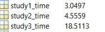
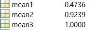
RESULTS: Time taken of the study ,global maxima value