Project 2 - Rankine cycle Simulator

AIM:- Creation of rankine cycle simulator from given input and reading tha data from standard thermodynamic library of steam table.

OBJECTIVE:-

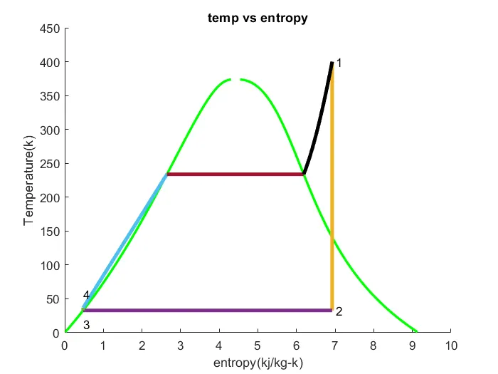
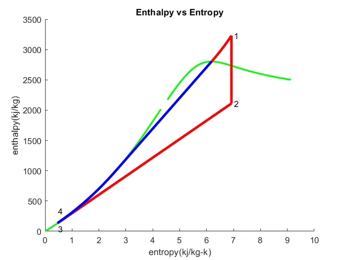
• To plot the T-s and H-S curve for given input in Rankine cycle.
• To get the output in command window for each state point in the cycle.
• To calculate the state point using function XSteam.

RANKINE CYCLE:- The Rankine cycle is an idealized themrodynamic cycle describing the process by which certain heat engines, such as steam turbine or reciprocating steam engines, allow mechanical work to be extracted from a fluid as it moves between a heat source and heat sink. The Rankine cycle is named after William John Macquorn Rankine.

Process 1–2: The working fluid is pumped from low to high pressure. As the fluid is a liquid at this stage, the pump requires little input energy. Process 1-2 is isentropic compression.

• Process 2–3: The high-pressure liquid enters a boiler, where it is heated at constant pressure by an external heat source to become a dry saturated vapour. The input energy required can be easily calculated graphically, using XSteam or software. Process 2-3 is constant pressure heat addition in boiler.
• Process 3–4: The dry saturated vapour expands through a turbine, generating power. This decreases the temperature and pressure of the vapour, and some condensation may occur. The output in this process can be easily calculated using the chart or tables noted above. Process 3-4 is isentropic expansion.
• Process 4–1: The wet vapour then enters a condensor, where it is condensed at a constant pressure to become a saturated liquid. Process 4-1 is constant pressure heat rejection in condenser.

MATLAB CODE

clear all 
close all
clc
disp('RANKINE CYCLE SIMULATOR');
disp('1-2=isentropic expansion in the turbine');
disp('2-3=constant pressure heat rejection in the condensor');
disp('3-4=isentropic compession in the pump');
disp('4-1= constant pressure heat addition by the boiler');

% To type the inputs and getting the text as given in the problem
disp('INPUTS')
t1=input('value of temperature at turbine inlet,(in degree celsius):');
p1=input('value of pressure at turbine inlet,p1(in bar):');
p2=input('value of pressure at condesor inlet,p2(in bar):');
 


 %stage 1 (turbine inlet)
 s1=XSteam('s_pT',p1,t1);
 h1=XSteam('h_pT',p1,t1);

 % stage 2 condensor inlet 
   s2=s1;
 sf2=XSteam('sL_p',p2);
 sg2=XSteam('sV_p',p2);
 x2=((s2-sf2)/(sg2-sf2));
 hf2=XSteam('hL_p',p2);
 hg2=XSteam('hV_p',p2);
 h2=hf2+(x2*(hg2-hf2));

 %stage 3
 p3=p2;
 s3=XSteam('sL_p',p3);
     h3=XSteam('hL_p',p3);

     %state 4
     s4=s3;
     p4=p1;

     % work done by turbine
     wt=h1-h2;
     v3=XSteam('vL_p',p3);
     wp=v3*(p4-p3)*100;
     h4=h3-wp;

     %net work
     wnet=wt-wp;
     %heat into the system
     Qin=h1-h4;
     %heat out of the system
     Qout=h2-h3;

     %thermal efficiency
     eff=(wnet/Qin)*100;

   %specific steam consumption
   SSc=(3600/wnet);
   %calculating temperature at the state points
   t3=XSteam('Tsat_p',p3);
   t2=t3;
   Cp4=XSteam('Cp_ps',p4,s4);
   Cv4=XSteam('Cv_ps',p4,s4);
   k=Cp4/Cv4;
   t4=t3/((p3/p4)^((k-1)/k));

   %calculating temperature,entropy,enthalpy at the vapour and liquid
   t6=XSteam('Tsat_p',p1);
   s5=XSteam('sL_p',p1);
   s6=XSteam('sV_p',p1);
   h5=XSteam('hL_p',p1);
   h6=XSteam('hV_p',p1);
   t5=t6;
    %plotting the saturation curve
    T=linspace(1,400,1000);
    for i=1:length(T)
  sf(i)=XSteam('sL_T',T(i));
  sg(i)=XSteam('sV_T',T(i));
   hf(i)=XSteam('hL_T',T(i));
   hg(i)=XSteam('hV_T',T(i));
    end

    %plotting T-S diagram
    figure(1)
    hold on
    plot(sf,T,'color','g','linewidth',2)
    plot(sg,T,'color','g','linewidth',2)
    plot([s1 s2],[t1 t2],'linewidth',3)
    plot([s2 s3],[t2 t3],'linewidth',3)
    plot([s3 s4],[t3 t4],'linewidth',3)
    plot([s4 s5],[t4 t5],'linewidth',3)
    plot([s5 s6],[t5 t6],'linewidth',3)

    sc1=linspace(s6,s1,1000);
    for l=1:length(sc1)
        Tc1(l)=XSteam('T_ps',p1,sc1(l));
    end
    plot(sc1,Tc1,'k','linewidth',3)
    text(s1+0.1,t1,'1')
    text(s2+0.1,t2,'2')
    text(s3,t3-20,'3')
    text(s4,t4+20,'4')
    title('temp vs entropy')
    xlabel('entropy(kj/kg-k)')
    ylabel('Temperature(k)')


%plotting H-S diagram
figure (2)
hold on 
plot(sf,hf,'color','g','linewidth',2)
plot(sg,hg,'color','g','linewidth',2)
plot([s1 s2],[h1 h2],'color','r','linewidth',3)
plot([s2 s3],[h2 h3],'color','r','linewidth',3)
plot([s3 s4],[h3 h4],'color','r','linewidth',3)
hc=linspace(h4,h5,100);
for k= 1:length(hc)
    sch(k)=XSteam('s_ph',p1,hc(k));
end
plot(sch,hc,'color','b','linewidth',3)
plot([s5 s6],[h5 h6],'color','b','linewidth',3)
for l = 1:length(sc1)
hc1(l)=XSteam('h_ps',p1,sc1(l));
end
plot(sc1,hc1,'color','r','linewidth',3)
text(s1+0.1,h1,'1')
text(s2+0.1,h2,'2')
text(s3,h3-100,'3')
text(s4,h4+200,'4')
title('Enthalpy vs Entropy')
xlabel('entropy(kj/kg-k)')
ylabel('enthalpy(kj/kg)')

%Displaying results in the command window
disp('RESULTS');
p1=p1;
t1=t1;
p3=p3;

disp('At state point 1');
p1=sprintf('p1 is %9f bar',p1);
disp(p1);
t1=sprintf('t1: %9f C',t1);
disp(t1);
h1=sprintf('h1: %9f Kj/kg',h1);
disp(h1);
s1=sprintf('s1: %9f Kj/Kg-k',s1);
disp(s1);

disp('At state point 2');
p2=sprintf('p2:%9f bar',p2);
disp(p2);
t2=sprintf('t2:%9f C',t2);
disp(t2);
h2=sprintf('h2:%9f Kj/kg',h2);
disp(h2);
s2=sprintf('s2:%9f Kj/Kg-k',s2);
disp(s2);

disp('At state point 3');
p3=sprintf('p3=%9f bar',p3);
disp(p3);
t3=sprintf('t3=%9f C',t3);
disp(t3);
h3=sprintf('h3=%9f Kj/kg',h3);
disp(h3);
s3=sprintf('s4=%9f Kj/Kg-k',s3);
disp(s3);

disp('At state point 4');
p4=sprintf('p4=%9f bar',p4);
disp(p4);
t4=sprintf('t4=%9f C',t4);
disp(t4);
h4=sprintf('h4=%9f Kj/kg',h4);
disp(h4);
s4=sprintf('s4=%9f Kj/Kg-k',s4);
disp(s4);

wt=sprintf('wt:%f Kj/kg',wt);
disp(wt);
wp=sprintf('wp:%fKj/kg',wp);
disp(wp);
wnet=sprintf('wnet:%f Kj/kg',wnet);
disp(wnet);
SSc=sprintf('SSc: %f Kj/KWh',SSc);
disp(SSc);

Explantaion:-

• clear all close all clc to erase the workspace .
• inputs variable p1 t1 p2 are given by input command .values are entered in command window while execute the code.
• state 1 value for enthalpy,entropy are extracted as afunction of preesure and temperature.
• h_pt,s_pt,hL_p,sV_p these values is stored in Xsteam file.
• state 2 condenser inlet where the high pressure steam is converted into low pressure water,enthalpy entropy for saturated water are considered to calculate the specific enthalpy.
• state 4 constant pressue heat addition ,pressure is equal to p1 but temperatue increase on heating at constant pressure and constant volume.
• entropy remains same and hence cp/cv=gamma.
• temperature range is defined using linspace command and for the overall lenghth of the temperature value of enthalpy and entropy are calculated at every temp.
• the break the saturation curve seprate the liquid phase &vapour phase.
• Now all the necessary data is found out,ploting is done of both T-S & H-S diagram using the plot command .
• assigned using text command.
• Results of the cycle simulation is displayed over command.
• using sprintf command.

RESULTS:-

T-S diagram

H-S diagram

OUTPUT IN COMMAND WINDOW:-

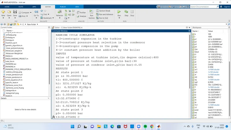
RANKINE CYCLE SIMULATOR
1-2=isentropic expansion in the turbine
2-3=constant pressure heat rejection in the condensor
3-4=isentropic compession in the pump
4-1= constant pressure heat addition by the boiler
INPUTS
value of temperature at turbine inlet,(in degree celsius):400
value of pressure at turbine inlet,p1(in bar):30
value of pressure at condesor inlet,p2(in bar):0.05
RESULTS
At state point 1
p1 is 30.000000 bar
t1: 400.000000 C
h1: 3231.571027 Kj/kg
s1:  6.923259 Kj/Kg-k
At state point 2
p2: 0.050000 bar
t2:32.875490 C
h2:2110.708212 Kj/kg
s2: 6.923259 Kj/Kg-k
At state point 3
p3= 0.050000 bar
t3=32.875490 C

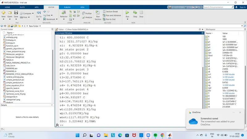
SCREENSHOT OF OUTPUT