Week 4.1 - Genetic Algorithm
AIM:
1. To write a code in MATLAB to optimise the stalagmite function and find the ‘Global Maxima’ of the function.
2. To explain the concept of genetic algorithm and also explain the syntax for ‘ga’ in MATLAB.
3. To plot graphs for all 3 studies and for function maximum vs number of iterations.
THEORY: Genetic Algorithm was first introduced by Holland in 1975, and it is a powerful stochastic search algorithm based on the mechanisms of natural genetics and selection. A general description of genetic algorithm is as follows:
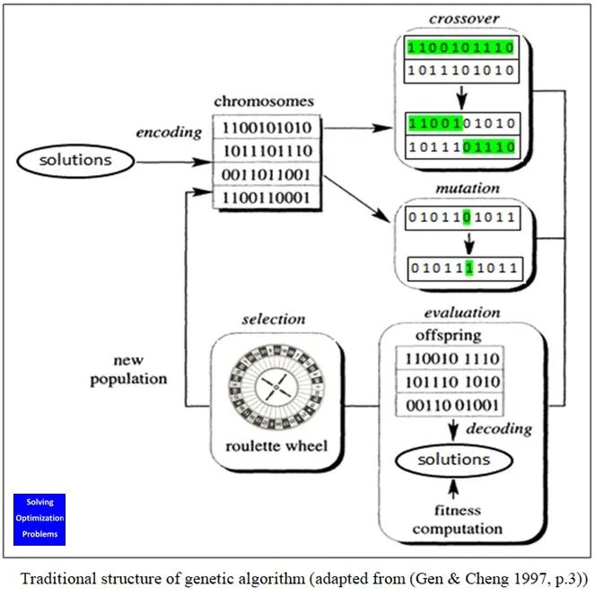
+ Genetic algorithm starts with an initial set of random solutions called population.
+ Each individual in the population is called a chromosome representing a solution to the problem at hand.
+ The chromosomes evolve through successive iterations, called generations.
+ During each generation, the chromosomes are evaluated using some measures of fitness.
+ To create the next generation, new chromosome, called offspring, are formed by either (a) merging two chromosomes from current generation using a crossover operator or (b) modifying a chromosome using a mutation operator.
+ A new generation is formed by (a) selecting, according to the fitness values, some of the parents and offspring and (b) rejecting others so as to keep the population size constant.
+ Fitter chromosomes have higher probabilities of being selected.
+ After several generations, the algorithms converge to the best chromosome, which hopefully represents the optimum or suboptimal solution to the problem.
Syntax:
x = ga(fun,nvars,A,b,Aeq,beq,lb,ub)
x = ga(fun,nvars,A,b,Aeq,beq,lb,ub,nonlcon)
x = ga(fun,nvars,A,b,Aeq,beq,lb,ub,nonlcon,options)
x = ga(fun,nvars,A,b,Aeq,beq,lb,ub,nonlcon,intcon)
x = ga(fun,nvars,A,b,Aeq,beq,lb,ub,nonlcon,intcon,options)
[x,fval,exitflag,output] = ga(___)
[x,fval,exitflag,output,population,scores] = ga(___)
Description:
x = ga(fun,nvars) finds a local unconstrained minimum, x, to the objective function, fun. nvars is the dimension (number of design variables) of fun.
x = ga(fun,nvars,A,b) finds a local minimum x to fun, subject to the linear inequalities A*x ≤ b. ga evaluates the matrix product A*x as if x is transposed (A*x').
x = ga(fun,nvars,A,b,Aeq,beq) finds a local minimum x to fun, subject to the linear equalities Aeq*x = beq and A*x ≤ b. (Set A=[] and b=[] if no linear inequalities exist.) ga evaluates the matrix product Aeq*x as if x is transposed (Aeq*x').
x = ga(fun,nvars,A,b,Aeq,beq,lb,ub) defines a set of lower and upper bounds on the design variables, x, so that a solution is found in the range lb ≤ x ≤ ub. (Set Aeq=[] and beq=[] if no linear equalities exist.)
x = ga(fun,nvars,A,b,Aeq,beq,lb,ub,nonlcon) subjects the minimization to the constraints defined in nonlcon. The function nonlcon accepts x and returns vectors C and Ceq, representing the nonlinear inequalities and equalities respectively. ga minimizes the fun such that C(x) ≤ 0 and Ceq(x) = 0. (Set lb=[] and ub=[] if no bounds exist.)
x = ga(fun,nvars,A,b,Aeq,beq,lb,ub,nonlcon,options) minimizes with the default optimization parameters replaced by values in options. (Set nonlcon=[] if no nonlinear constraints exist.) Create options using optimoptions.
x = ga(fun,nvars,A,b,Aeq,beq,lb,ub,nonlcon,intcon) or x = ga(fun,nvars,A,b,Aeq,beq,lb,ub,nonlcon,intcon,options) requires that the variables listed in intcon take integer values.
x = ga(problem) finds the minimum for problem, a structure described in problem.
[x,fval] = ga(___), for any previous input arguments, also returns fval, the value of the fitness function at x.
[x,fval,exitflag,output] = ga(___) also returns exitflag, an integer identifying the reason the algorithm terminated, and output, a structure that contains output from each generation and other information about the performance of the algorithm.
[x,fval,exitflag,output,population,scores] = ga(___) also returns a matrix population, whose rows are the final population, and a vector scores, the scores of the final population.
MATLAB CODE:
clear all
close all
clc

x = linspace(0,0.6,150);
y = linspace(0,0.6,150);
num_cases = 150
[xx yy] = meshgrid(x,y);

for i = 1:length(xx)
    for j = 1:length(yy)
        input_vector(1) = xx(i,j);
        input_vector(2) = yy(i,j);
        F(i,j) = stalagmite(input_vector);
    end
end

% Study 1 - Statistical Behavior
tic
for i = 1:num_cases
    [inputs, fopt(i)] = ga(@stalagmite,2);
    xopt(i) = inputs(1);
    yopt(i) = inputs(2);
end

study1_time = toc


subplot(2,1,1)         % Making subplots in figure(1)
surfc(xx,yy,-F)
hold on
shading interp         % To smoothen the plot
plot3(xopt,yopt,-fopt,'marker','o','MarkerSize',5,'MarkerFaceColor','r')  % Making a 3D plot
title('Unbounded inputs')
xlabel('X Axis')
ylabel('Y Axis')
subplot(2,1,2)
plot(-fopt)
xlabel('Iterations')
ylabel('Function Maxima')

% Study 2 - Statistical Behavior with Upper and Lower bounds
tic
for i = 1:num_cases
    [inputs2, fopt2(i)] = ga(@stalagmite,2,[],[],[],[],[0,0],[1,1]);
    xopt2(i) = inputs2(1);
    yopt2(i) = inputs2(2);
end
study2_time = toc

figure(2)

subplot(2,1,1)
surfc(xx,yy,-F)
hold on
shading interp
plot3(xopt2,yopt2,-fopt2,'marker','o','MarkerSize',5,'MarkerFaceColor','r')
title('Bounded inputs')
xlabel('X Axis')
ylabel('Y Axis')
subplot(2,1,2)
plot(-fopt2)
xlabel('Iterations')
ylabel('Function Maxima')

% Study 3 - Increasing 'ga' iteratiions

options = optimoptions('ga');
options = optimoptions(options,'PopulationSize',500);

tic
for i = num_cases
    [inputs3, fopt3(i)] = ga(@stalagmite,2,[],[],[],[],[0,0],[0.6,0.6],[],[],options);
    xopt3(i) = inputs3(1);
    yopt3(i) = inputs3(2);
end
study3_time = toc

figure(3)

subplot(2,1,1)
surfc(xx,yy,-F)
hold on
shading interp
plot3(xopt3,yopt3,-fopt3,'marker','o','MarkerSize',5,'MarkerFaceColor','r')
title('Bounded inputs with Population size as 500')
xlabel('X Axis')
ylabel('Y Axis')
subplot(2,1,2)
plot(-fopt3)
xlabel('Iterations')
ylabel('Function Maxima')
FUNCTION CODE:
function [F] = stalagmite(input_vector)
x = input_vector(1);
y = input_vector(2);

F1_x = (sin(5.1*pi*x+0.5))^6;
F1_y = (sin(5.1*pi*y+0.5))^6;
F2_x = exp(-4*log(2)*((x-0.0667)^2/(0.64)));
F2_y = exp(-4*log(2)*((y-0.0667)^2/(0.64)));

F = -(F1_x*F1_y*F2_x*F2_y)
end
EXPLANATION:
+ We start with clear all, close all and clc command to clear all the previous data.
+ x and y value has been provided using linspace command and iteration of 50 times have been set by saying
num_cases is equal to 150.
+ Meshgrid command is used to convert the 1D array of x and y to 2D array of xx and yy.
+ For loop is used for the full length of xx and yy and the input function was used which is a row vector with two
coloum assigned as input-vector(1) and input_vector(2).
+ We created a stalagmite function to find the local maxima and minima. After creating it, we called this function
program into our main program.
+ The formula which was used in the stalagmite function is of two variables i.e. x and y. The formula is shown below.
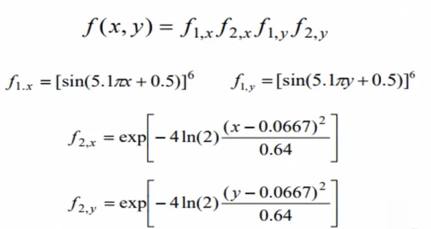
+ Here in the above formula, we can see that F(x,y) is the output and we used input_vector(1) and (2) as x and y
inputs. Since, we knew that 'ga' command using stalagmite function will only give us the global minima, so in
order to get the global maxima which was asked in the objective, we need to multiply the output function with
(-1).
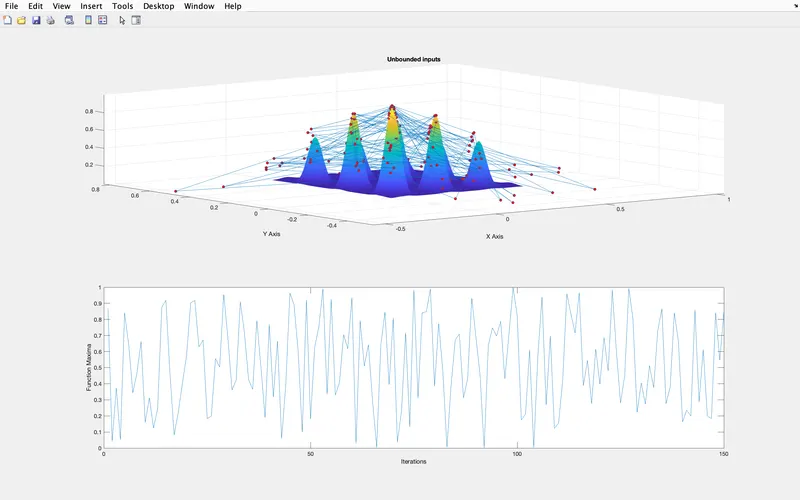
+ Now, for the study 1 - statistical behaviour, we are making it free with no bounds and just making it
the population size of 50.
+ Here, we used the following syntax- [inputs, fopt(i)] = ga(@stalagmite,2); which we understand before as
[x,fval] = ga(___), for any previous input arguments, also returns fval, the value of the fitness function at x. And
we run a for loop for iterative of 50 cases. Here, the variables used is 2 and we used tic and toc command to
measure the study time for study 1. @
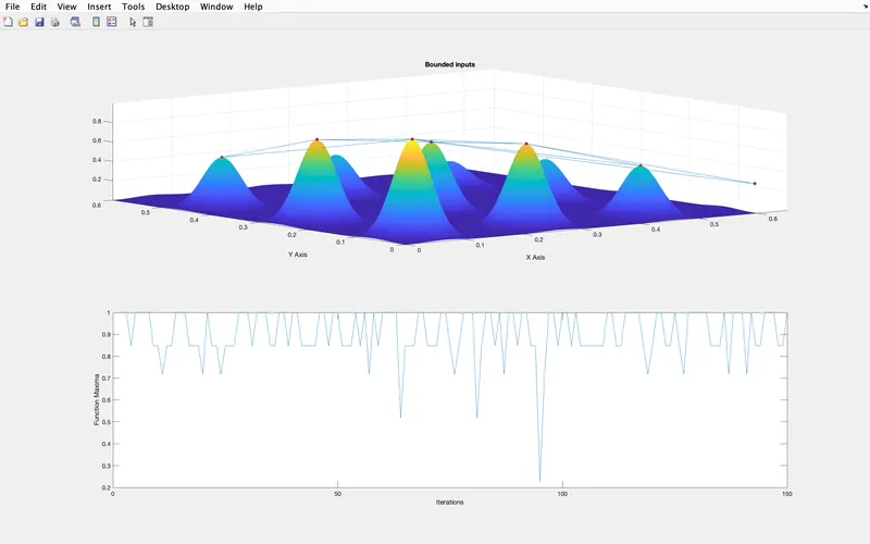
+ In the second study i.e. study 2 - statistical behaviour with upper and lower bounds this time and we used the
syntax - [inputs, fopt(i)] = ga(@stalagmite,2,[],[],[],[],[0;0],[1;1]); and did the same loop as study 1.
+ In the third study i.e. study 3 - increasing the population with upper and lower bounds, we used the syntax-
[inputs, fopt(i)] = ga(@stalagmite,2,[],[],[],[],[0;0],[1;1],[],[],options);. For this we set the population size of
300 and used the loop.
+ We used tic and toc command in every study we mentioned above to measure the study time for each study,
in which we find study1 took 4.8992sec, study2 took 7.9142sec and study3 took 0.3989 sec. Here, we can
understand that study1 had no bounds so it took more time, then in study2 we make a bound, so that it can
take search the global maxima in a region and then in study3, we just increase the population size. @
+ Now for plotting, we are plotting 2 graphs one is in 3D and another in 2D by applying subplot and using plot3 and
plot. Shading interp is used so that the graph would be more representable and smooth. we used this plot in all
the three studies mentioned above and the output graphs that we found is presented below.
Study1 OUTPUT-
Study 2 OUTPUT-
Study 3 OUTPUT-
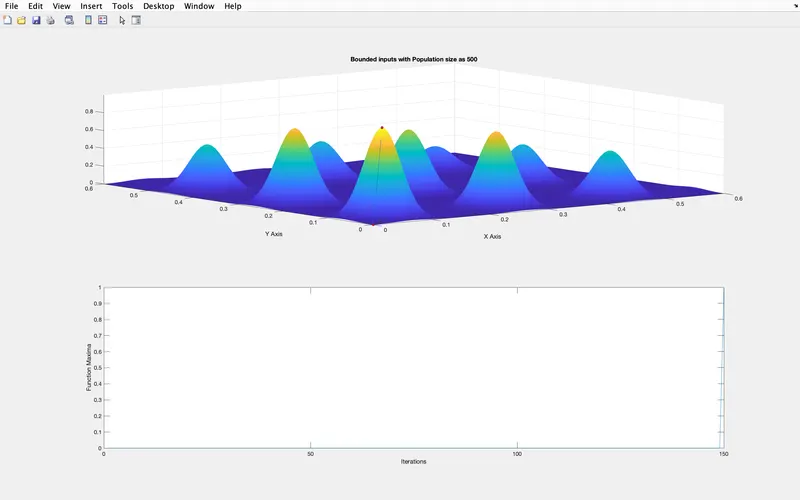
+ As a result, we trying to get minimum global maxima value so that we can achieve the best possible result by optimization.
+ Submitting the output result in screenshot format.
ERROR: Did a mistake while writing the formula of F1_x and F1_y and as a result I got this plot:-
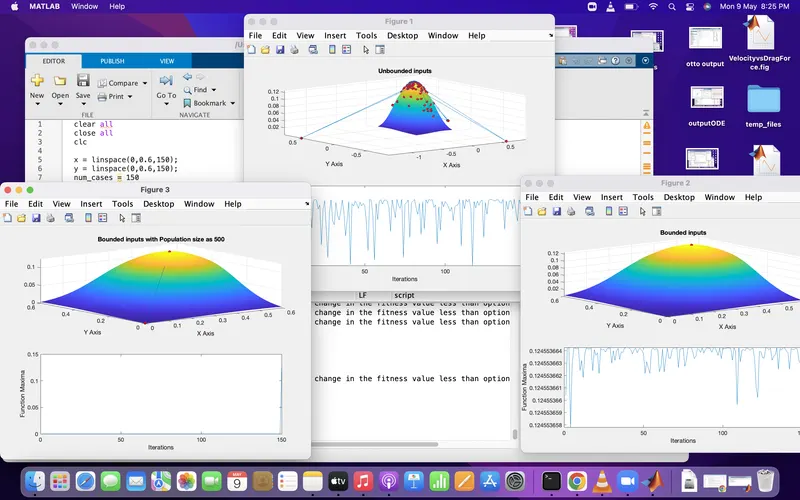
Have to correct the formula to get the right result.
REFERENCE: