Week 3 - Solving second order ODEs

AIM: To write a program in Matlab that will simulate the Pendulum motion.

OBJECTIVE: To solve a second order ODE, which represents equation of motion of a simple pendulum with damping and create an animated video with output obtained from solving ODE.

THEORY: A simple pendulum is a mechanical system of mass attached to a long massless inextensible string with a bob attached to it that performs oscillatory motion.

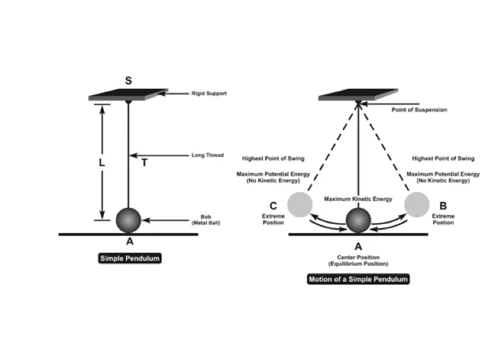
The way the pendulum moves depends on the Newtons second law. When this law is written down, we get a second order Ordinary Differential Equation that describes the position of the "ball" w.r.t time.

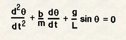
In the above equation,

g = gravity in m/s2

L = length of pendulum in m

m = mass of the bob in kg

b = damping coefficient

Code:

% Program in Matlab that will simulate the pendulum motion
clear all
close all
clc
b = 0.05;     % Damping Coefficient
g = 9.81;     % Gravity (m/s^2)
L = 1;        % Length of the string (m)
m = 1;        % Mass of the bob (kg)

% Initial condition
theta_0 = [0;3];      % [Angular displacement(rad) ; Angular velocity(rad/s)]

% Time points
t_span = linspace(0,20,150);   % Integrating time (s)

% Solving ODE through ode45, an inbuilt function in matlab
[t,results] = ode45(@(t,theta)ode_func(t,theta,b,g,L,m),t_span,theta_0);

% Plotting
plot(t,results(:,1),'LineWidth',3)
hold on
plot(t,results(:,2),'LineWidth',3)
xlabel('time')
ylabel('Plot')
legend('Angular displacement','Angular velocity')
grid on

% Using for loop to create an animation of simple pendulum
ct = 1;

for i = 1:length(t)

% Initial Coordinates
    x0 = 0;
    y0 = 0;

% Final Coordinates
    x_end = L * sin(results(i,1));
    y_end = -L * cos(results(i,1));

    % Plotting for animation

    % Base of Pendulum
    figure(2)
    plot([-1 1],[0 0],'linewidth',4,'Color','black')
    hold on
    plot(x0,y0,'Marker','o','MarkerSize',6,'Color','y')

    % String of Pendulum
    plot([x0 x_end],[y0 y_end],'linewidth',6,'Color','b')
    hold on

    % Bob of Pendulum
    plot(x_end, y_end,'Marker','o','MarkerSize',28,'MarkerFaceColor','r')

    title('damping of simple pendulum')
    legend('support bar','fixed point','length of string','bob of pendulum')
    
    axis ([-2 2 -2 2])
    grid on
    pause(0.11)
    hold off;
    M(ct) = getframe(gcf);     % Gathering all frames together
    ct = ct+1;
end

% Creating an animation
movie(M)
videofile = VideoWriter('Simple_Pendulum.avi','Uncompressed AVI');
open(videofile);
writeVideo(videofile,M);
close(videofile);

Code for ode45 function in program

function [dtheta_dt] = ode_func(t,theta,b,g,L,m)
theta1 = theta(1)
theta2 = theta(2)

dtheta1_dt = theta2;
dtheta2_dt = -(b/m)*theta2-(g/L)*sin(theta1);
dtheta_dt = [dtheta1_dt ; dtheta2_dt];


end

WORKING:

1. At first, we created a function program separately to solve ODE in matlab, in which since the given equation is in Second order differential equation, so, we changed it into First order by-

dtheta1_dt = theta2 and dtheta2_dt = -(b/m)*theta2-(g/L)*sin(theta1).

2. After creating the function for ODE, in the new script, we first include all the inputs mainly damping coefficient, gravity, length of string and mass of bob.

3. We have also provided the initial angular displacement and velocity and also included the time span.

4. Calling the function program to solve the ODE using matlab inbuilt function I.e. ode45, used with ’t’ and ‘theta’ which is dependent and independent variable.

5. Plotting a graph of both angular displacement and velocity with respect to time using hold on command.

6. Iteration of coordinates is provided using ‘for loop’ to create an animation in the figure(2).

7. Used ‘Marker’ command to make the bob of the pendulum.

8. We used plot command to make the base, string and bob of the pendulum. Also provided the axis. Then, used get frame command to gather all the frames together and make an animation.

9. Movie command is used to create a movie and posted in YouTube with link https://youtu.be/OGt0rO5XvV4 .

OUTPUT: Output obtained posted in the form of picture.

1. Mistake : Forget to use hold on command.

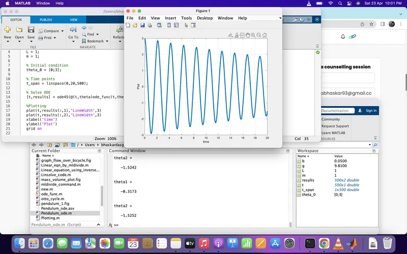
2. Mistake: Used sind and cosd values in degree. As a result, my bob was not moving far enough due to less values of theta. As soon as I changed it to sin and cos in radian, my bob was moving at distance.

CONCLUSION: The simulation of simple pendulum is created successfully using Second order differential equation.