Week 4.1 - Genetic Algorithm
Code to optimise the stalagmite function and find the global maxima of the function.
clear all
close all
clc
x = linspace(0,0.6,50)
y = linspace(0,0.6,50)
[xx yy] = meshgrid(x,y)
for i = 1:length(xx)
    for j =1:length(yy)
        input_vector(1)=xx(i,j)
        input_vector(2)= yy(i,j)
        f(i,j) = stalagmite(input_vector)
    end
end
F = -f
surfc(xx,yy,f)
hold on
[output ,fval] = ga(@stalagmite, 2,[],[],[],[],[0,0],[0.6,0.6])

xmax = output(:,1)
ymax = output(:,2)
fmax = -fval
plot(xmax,ymax,fmmax,'marker','o','markersize',5,'markerfacecolor','r')
xlabel('x value')
ylabel('y value')
title('Global Maxima')
legend('Stalagmite','Global Maxima')
Step-wise explanation of your code
- First we will use clear all, close all and clc command.
- Now assigning the value of x and y using linspace command.
- Now using the meshgrid command to make 2D array.
- Now using the for loop and inserting the value of input vector.
- Now putting the stalagmite function values.
- For finding the global maxima putting negative sign on stalagmite function.
- Now using the surface command to creat 3D plot.
- Getting the value of ymax,xmax and fmax.
- Now plotting the above values.
- Now using xlabel , ylabel, title and legend command.
The errors faced while programming was I putting the equations for stalagmite function and to solve this problem I was rechecking the code and was paying attention.

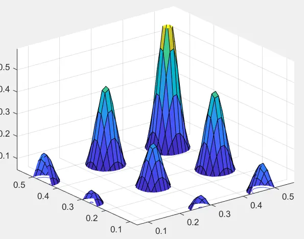
STALAGMITE - A stalagmite is an upward-growing mound of mineral deposits that have precipitated from water dripping onto the floor of a cave. Most stalagmites have rounded or flattened tips.
GENETIC ALGORITHM
The genetic algorithm (GA), developed by John Holland and his collaborators in the 1960s and 1970s (Holland, 1975; De Jong, 1975), is a model or abstraction of biological evolution based on Charles Darwin's theory of natural selection.Genetic Algorithms(GAs) are adaptive heuristic search algorithms that belong to the larger part of evolutionary algorithms. Genetic algorithms are based on the ideas of natural selection and genetics. These are intelligent exploitation of random search provided with historical data to direct the search into the region of better performance in solution space. They are commonly used to generate high-quality solutions for optimization problems and search problems.
Genetic algorithms simulate the process of natural selection which means those species who can adapt to changes in their environment are able to survive and reproduce and go to next generation. In simple words, they simulate “survival of the fittest” among individual of consecutive generation for solving a problem. Each generation consist of a population of individuals and each individual represents a point in search space and possible solution. Each individual is represented as a string of character/integer/float/bits. This string is analogous to the Chromosome.
The five phases which are considered in a genetic algorithm.
- Initial population
- Fitness function
- Selection
- Crossover
- Mutation
Initialisation
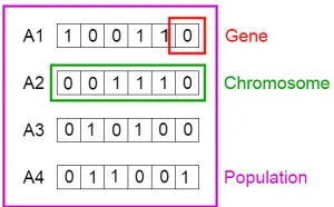
To solve this problem using genetic algorithm, our first step would be defining our population. So our population will contain individuals, each having their own set of chromosomes.
We know that, chromosomes are binary strings, where for this problem 1 would mean that the following item is taken and 0 meaning that it is dropped.
Fitness Function
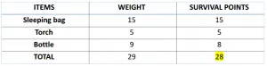
Let us calculate fitness points for our first two chromosomes.
For A1 chromosome [100110],
imilarly for A2 chromosome [001110],
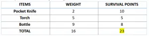
So, for this problem, our chromosome will be considered as more fit when it contains more survival points.
Therefore chromosome 1 is more fit than chromosome 2.
Selection
Now, we can select fit chromosomes from our population which can mate and create their off-springs.
General thought is that we should select the fit chromosomes and allow them to produce off-springs. But that would lead to chromosomes that are more close to one another in a few next generation, and therefore less diversity.
Therefore, we generally use Roulette Wheel Selection method.
Don’t be afraid of name, just take a look at the image below.

Crossover
So in this previous step, we have selected parent chromosomes that will produce off-springs. So in biological terms, crossover is nothing but reproduction.
So let us find the crossover of chromosome 1 and 4, which were selected in the previous step. Take a look at the image below.
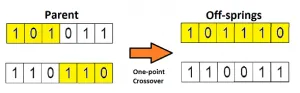
This is the most basic form of crossover, known as one point crossover. Here we select a random crossover point and the tails of both the chromosomes are swapped to produce a new off-springs.
Mutation
Now if you think in the biological sense, are the children produced have the same traits as their parents? The answer is NO. During their growth, there is some change in the genes of children which makes them different from its parents.
This process is known as mutation, which may be defined as a random tweak in the chromosome, which also promotes the idea of diversity in the population.
A simple method of mutation is shown in the image below.

TO GENERATE STALAGMITE FUNCTION BELOW FUNCTION IS USED-
f1=(sin(5.1*pi*x+0.5))^6;
f2=(sin(5.1*pi*y+0.5))^6;
f3=exp(-4*log(2)*((x-0.667)^2)/0.64);
f4=exp(-4*log(2)*((y-0.667)^2)/0.64);
f=f1*f2*f3*f4;
Syntax of ga
DESCRIPTIONx = ga(fun,nvars) finds a local unconstrained minimum, x, to the objective function, fun. nvars is the dimension (number of design variables) of funx = ga(fun,nvars,A,b,Aeq,beq,lb,ub,nonlcon)nonlcon. The function nonlcon accepts x and returns vectors C and Ceq, representing the nonlinear inequalities and equalities respectively. ga minimizes the fun such that C(x) ≤ 0 and Ceq(x) = 0. (Set lb=[] and ub=[] if no bounds exist.)
x = ga(fun,nvars,A,b,Aeq,beq,lb,ub,nonlcon,options)options. (Set nonlcon=[] if no nonlinear constraints exist.) Create options using optimoptions.
x = ga(fun,nvars,A,b,Aeq,beq,lb,ub,nonlcon,intcon)x = ga(fun,nvars,A,b,Aeq,beq,lb,ub,nonlcon,intcon,options)intcon take integer values
Code for all 3 studies
clear all
close all
clc
x = linspace(0,0.6,150);
y = linspace(0,0.6,150);
[xx,yy] = meshgrid(x,y);
num_cases = 20;
for i = 1:length(xx)
    for j= 1:length(yy)
        input_vector(1)=xx(i,j);
        input_vector(2)=yy(i,j);
        f(i,j)= get_stalagmite(input_vector);
    end
end

for i = 1:num_cases
    [inputs, fopt(i)] = ga(@get_stalagmite, 2);
    xopt(i) = inputs(1);
    yopt(i) = inputs(2);
end
fopt=-fopt;
figure(1)
subplot(2,1,1)

surfc(x,y,-f)
shading interp
hold on
plot3(xopt,yopt,fopt,'marker','o','markersize',5,'markerfacecolor','r')
title('Unbounded inputs')
subplot(2,1,2)
plot(fopt)
xlabel('Iterations')
ylabel('Function minimum')
tic
%Study 2 -Statistical behavior - with upper and lower bound
for i = 1:num_cases
[inputs2, fopt2(i)] = ga(@get_stalagmite, 2,[],[],[],[],[0;0],[0.4;0.4]);
xopt2(i) = inputs2(1);
yopt2(i) = inputs2(2);
end
fopt2 = -fopt2;
study2_time = toc;
figure(2)
subplot(2,1,1)

surfc(x,y,-f)
shading interp
hold on
plot3(xopt2,yopt2,fopt2,'marker','o','markersize',5,'markerfacecolor','r')
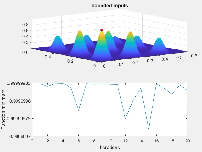
title('bounded inputs')
subplot(2,1,2)
plot(fopt2)
xlabel('Iterations')
ylabel('Function minimum')
% Study 3 increasing GA iterations
options = optimoptions('ga');
options = optimoptions(options,'populationsize',200);
tic
for i = 1:num_cases
   [inputs3, fopt3(i)] = ga(@get_stalagmite,2,[],[],[],[],[0;0],[0.4;0.4],[],[],options);
    xopt3(i) = inputs3(1);
    yopt3(i) = inputs3(2);
end
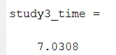
study3_time = toc
figure(3)
subplot(2,1,1)

surfc(x,y,-f)
shading interp
hold on
plot3(xopt3,yopt3,-fopt3,'marker','o','markersize',5,'markerfacecolor','r')
title('bounded inputs')
subplot(2,1,2)
plot(-fopt3)
xlabel('Iterations')
ylabel('Function minimum')
Figure1
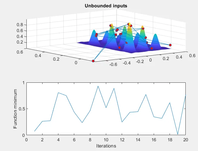
Figure 2
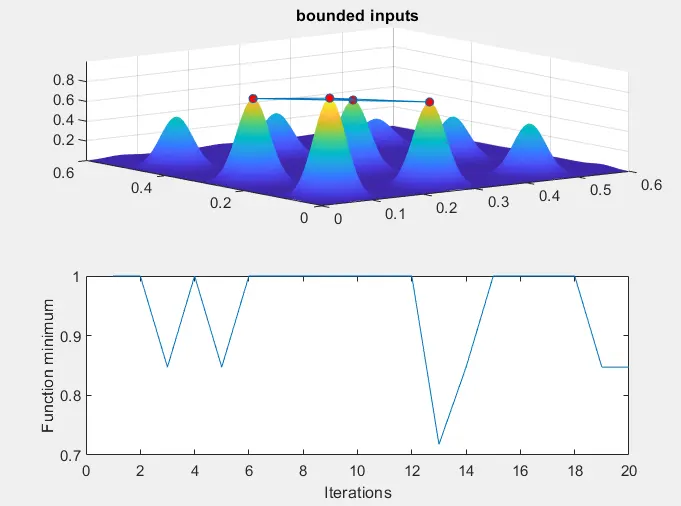
Figure 3
Command Window
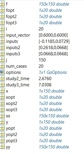
Workspace