Genetic Algorithm
1. AIM : Write a code in MATLAB to optimise the stalagmite function and find the global maxima of the function.
2. GOVERNNING EQUATION :
- Stalagmite Mathematical Modle function ( Fitness Function ) :
`f(x,y)= f_1x*f_2x * f_1y * f_2y`
`f_1x = [sin(5.1pix+0.5)]^6` ; `f_1y=[sin(5.1piy+0.5)]^6`
`f_2x = exp[-4ln(2)frac((x-0.0667)^2)(0.64)]`
`f_2y=exp[-4ln(2)frac((y-0.0667)^2)(0.64)]`
where, x & y are the input variable.
This been obtained just using nonlinear regression analysis. The name came to the function because it resembles as a stalagmite rock formation.
- Inbuilt mathematical functions used to perform GA :
[ x , fval ] = ga ( ___ )
[ x , fval ] = ga ( fun , nvars , A , b , Aeq , beq , lb , ub )
[ x , fval ] = ga(fun,nvars,A,b,[],[],lb,ub,nonlcon,IntCon,options)
3. OBJECTIVES OF THE FUNCTION :
- Optimize the Stalagmite function Using a "Genetic Algorithm"(GA) method & find the Global maxima.
- Plot graphs for F maximum vs no. of iterations.
4. BODY OF THE CONTENT :
GENETIC ALGORITHM CONCEPT :
The genetic algorithm is a random-based classical evolutionary algorithm.GA is based on Darwin’s theory of evolution. It's doing simply a mimic of 'natural genetic population selection'.
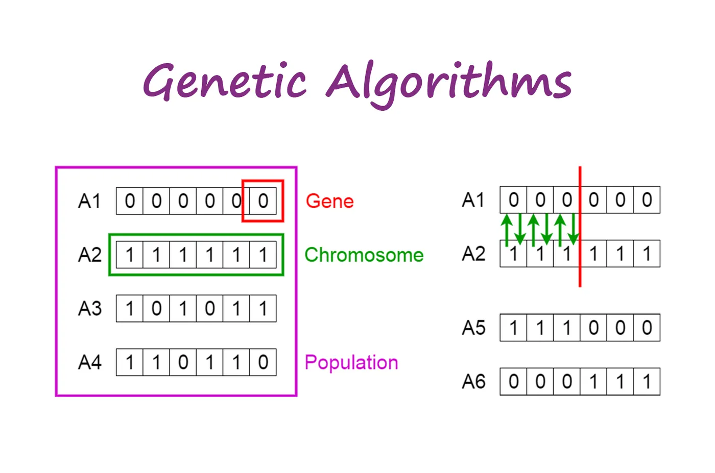
There are some phases that we can considered in a genetic algorithm :
- Initial population :
The process begins with a set of individuals which is called a Population. Each individual is a solution to the problem you want to solve. An individual is characterized by a set of parameters (variables) known as Genes. Genes are joined into a string to form a Chromosome (solution).
2. Fitness Function :
Here the fitness function ( also known as the Evaluation Function ) determines how fit an individual is. In genetic algorithms, each solution is generally represented as a string of binary numbers, known as a chromosome. We have to test these solutions and come up with the best set of solutions to solve a given problem.
3. Selection :
Selection is the stage of a genetic algorithm in which individual genomes are chosen from a population (using the crossover operator).
4. Crossover :
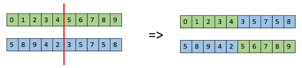
Crossover is a genetic operator used to vary the programming of a chromosomes from one generation to the next. Crossover is sexual reproduction. Two strings are picked from the mating pool at random to crossover in order to produce superior offspring. The method chosen depends on the Encoding Method, Like One Point Crossover, Two or Multi Point Crossover, Uniform Crossover. Here one of them explained.
One Point Crossover :
In this one-point crossover, a random crossover point is selected and the tails of its two parents are swapped to get new off-springs.
5. Mutation :
Mutation is a genetic operator used to maintain genetic diversity from one generation of a population of genetic algorithm chromosomes to the next.The mutation of bit strings ensue through bit flips at random positions.
Example:
` 1 0 1 0 0 1 0`
` ↓`
` 1 0 1 0 1 1 0`
The probability of a mutation of a bit is `frac (1)(l)` where `l` is the length of the binary vector.
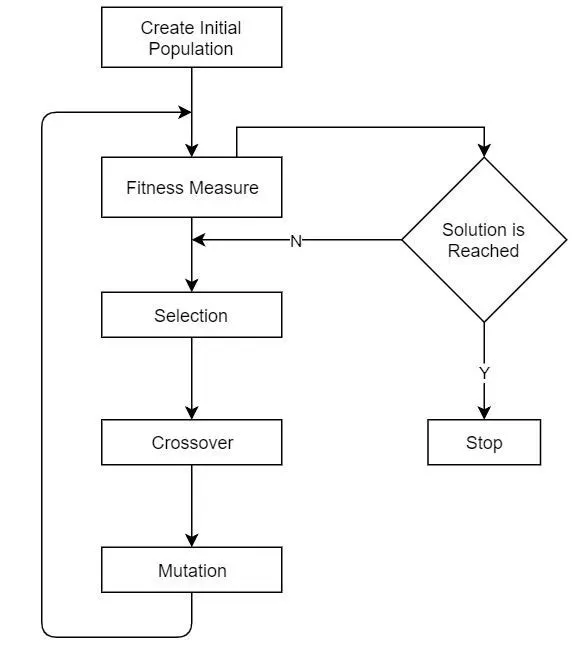
GA flow chart
5. MATLAB Code :
Stalagmite Mathematical Modle function ( Fitness Function )
% Stalagmite Mathematical Modle function ( Fitness Function )

function [f]= stalagmite(input_vector)
f1_x = (sin(5.1*pi*input_vector(1) + 0.5))^6;
f1_y = (sin(5.1*pi*input_vector(2) + 0.5))^6;
f2_x = exp((-4*log(2)*((input_vector(1)-0.0667)^2/(0.64))));
f2_y = exp((-4*log(2)*((input_vector(2)-0.0667)^2/(0.64))));
f = -(f1_x*f1_y*f2_x*f2_y);     % '-' sign inserted to find a globle maxima
end
# INPUT :
% Write a code in MATLAB to optimise the stalagmite function and find the global maxima of the function.
% Performing GA optimisation process on "Stalagmite Mathematical Modle function ( Fitness Function )"

clear all
close all
clc

x = linspace(0,0.6,150);            % taken higher number(150) of point, to see graph more smoother
y = linspace(0,0.6,150);
num_cases = 50 ;                     % number of iteration

[XX,YY]= meshgrid(x,y);         % Creating a 2Dimensional mesh


% Evaluating the stalagmite function
% Generating the data for z-axis( f values) to vizulizing the stalagmite function
for i = 1:length(XX)            % run loop for """size of 'XX' matrix""" number of times
    for j = 1: length(YY)       % run loop for """size of 'YY' matrix""" number of times
        input_vector(1) = XX(i,j);       % extracting 'XX' matrix value "one value at a time" on each run of loop
        input_vector(2) = YY(i,j);       % extracting 'YY' matrix value "one value at a time" on each run of loop
        f(i,j) = -stalagmite(input_vector);    % sequentially putting value of 'inpit_vector' & generate 'f'(z-axis)value corresponding 'XX'&'YY' data.
    end                                        % '-' inserted to get globle maxima
end
%%

%%
%%%%%%%%%%%%%%%%%%%%%%%%%%%%     Study - 1, Statistics behavior     %%%%%%%%%%%%%%%%%%%%%%%%%%%%%

tic                          % Starting time to calculate time of Study 1
for k = 1 : num_cases        % run ga@function for number of 'num_cases' & collecting each values on each run.
    [inputs, fopt(k)] = ga(@stalagmite, 2 );    % [x,fval] = ga(___), where x = Solution, & fval = Objective function value at the solution
    xopt(k) = (inputs(1));                      % taking x-optimum value from 'inputs'
    yopt(k) = (inputs(2));                      % taking y-optimum value from 'inputs'
    zopt(k) = -(fopt(k));                       % taking z-optimum value from 'fopt()'  %% '-' sign inserted to show valuse in z(positive) direction
end
Study_1_time_taken = toc                        % End command, to calculate time of Study 1

% plotting study 1 results
figure('Name',"   Study - 1 Statistics behavior",'NumberTitle','on')    % applying name to figure window

subplot(2,1,1)              % subplot 1 at top position
hold on
surfc(XX,YY,f)              % visualizing the stalagmite function in 3d
shading interp              % removing mesh in surface plot
plot3(xopt,yopt,zopt,'marker','o','markersize',5)      % plloting  the "ga" prediction values
title('Study - 1 Statistics behavior (Unbounded inputs)')
xlabel('XX & xopt')         % giving name to x axis
ylabel('YY & yopt')         % giving name to y axis
zlabel('f & zopt')          % giving name to z axis
legend('visualization of stalagmite function','','"ga" prediction values','Location','southeast')

subplot(2,1,2)              % subplot 2 at bottom position
plot(zopt)                  % plotting function[f] value vs number of intresion
xlabel('Iterations')        % giving name to x axis
ylabel('Function maximum')  % giving name to y axis
legend('function[f] value')
saveas(figure(1),'Study_1_Statistics_behavior.png')

hold off
%%


%%
%%%%%%%%%%%%%%%%%%%%%%%%%% Study 2 - Statistical behavior - with upper & lower bounds   %%%%%%%%%%%%%%%%%%%%%%%%%%%%%%%%%

tic                         % Starting  time to calculate time of Study 2
for m = 1:num_cases         % run ga@function for number of 'num_cases' & collecting each values on each run.
    [inputs, fopt(m)] = ga(@stalagmite,2,[],[],[],[],[0;0],[1;1]);  % definding lower & upper limits,where [x,fval] = ga(fun,nvars,A,b,Aeq,beq,lb,ub)
    xopt(m) = (inputs(1));  % taking x-optimum value from 'inputs'
    yopt(m) = (inputs(2));  % taking y-optimum value from 'inputs'
    zopt(m) = -(fopt(m));   % taking z-optimum value from 'fopt()'  %% '-' sign inserted to show valuse in z(positive) direction
end
Study_2_time_taken = toc    % End command, to calculate time of Study 2

% plotting Study 2 result
figure('Name',"   Study 2 - Statistical behavior - with upper & lower bounds",'NumberTitle','on')    % applying name to figure window

subplot(2,1,1)              % subplot 1 at top position
hold on
surfc(XX,YY,f)              % visualizing the stalagmite function in 3d
shading interp              % removing mesh in surface plot
plot3(xopt,yopt,zopt,'marker','o','markersize',5)   % plloting  the "ga" prediction values
title('Study 2 - Statistical behavior with upper-lower bounds (Bounded inputs)')
xlabel('XX & xopt')         % giving name to x axis
ylabel('YY & yopt')         % giving name to y axis
zlabel('f & zopt')          % giving name to z axis
legend('visualization of stalagmite function','','"ga" prediction values')

subplot(2,1,2)              % subplot 2 at bottom position
plot(zopt)                  % plotting function[f] value vs number of intresion
xlabel('Iterations')        % giving name to x axis
ylabel('Function maximum')  % giving name to y axis
legend('function[f] value')
saveas(figure(2),'Study_2_Statistics_behavior_with_upper_and_lower_bounds.png')
hold off
%%


%%
%%%%%%%%%%%%%%%%%%%%%%%%%%%      Study 3 - Incresing GA iterations      %%%%%%%%%%%%%%%%%%%%%%%%%%%%%%

tic                         % Starting  time to calculate time of Study 3
options = optimoptions('ga');   % where, options = optimoptions(SolverName)-
                                % -returns a set of default options for the 'ga' solver.
options = optimoptions(options,'PopulationSize',150);   % where, options = optimoptions(SolverName,Name,Value)-
                                % -returns options with specified parameters set using PopulationSize.


for n = 1 : num_cases       % run ga@function for number of 'num_cases' & collecting each values on each run.
    [inputs,fopt(n)] = ga (@stalagmite,2,[],[],[],[],[0;0],[1;1],[],[],options);
                            % where, [x,fval] = ga(fun,nvars,A,b,[],[],lb,ub,nonlcon,IntCon,options)
    xopt(n) = inputs(1);    % taking x-optimum value from 'inputs'
    yopt(n) = inputs(2);    % taking y-optimum value from 'inputs'
    zopt(n) = -(fopt(n));   % taking z-optimum value from 'fopt()'  %% '-' sign inserted to show valuse in z(positive) direction
end
Study_3_time_taken = toc    % End command, to calculate time of Study 3

% plotting Study 3 result
figure('Name',"   Incresing GA iterations ",'NumberTitle','on')    % applying name to figure window

subplot(2,1,1)              % subplot 1 at top position
hold on
surfc(XX,YY,f)              % visualizing the stalagmite function in 3d
shading interp              % removing mesh in surface plot
plot3(xopt,yopt,zopt,'marker','o','markersize',5 )   % plloting  the "ga" prediction values
title('Study-3 Incresing GA iterations (Bounded inputs)')
xlabel('XX & xopt')         % giving name to x axis
ylabel('YY & yopt')         % giving name to y axis
zlabel('f & zopt')          % giving name to z axis
legend('visualization of stalagmite function','','"ga" prediction values')

subplot(2,1,2)              % subplot 2 at bottom position
plot(zopt)                  % plotting function[f] value vs number of intresion
xlabel('Iterations')        % giving name to x axis
ylabel('Function maximum')  % giving name to y axis
legend('function[f] value')
saveas(figure(3),'Study_3_Incresing_GA_iterations.png')
hold off

%%
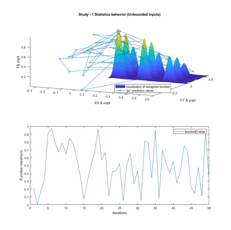
# OUTPUT :
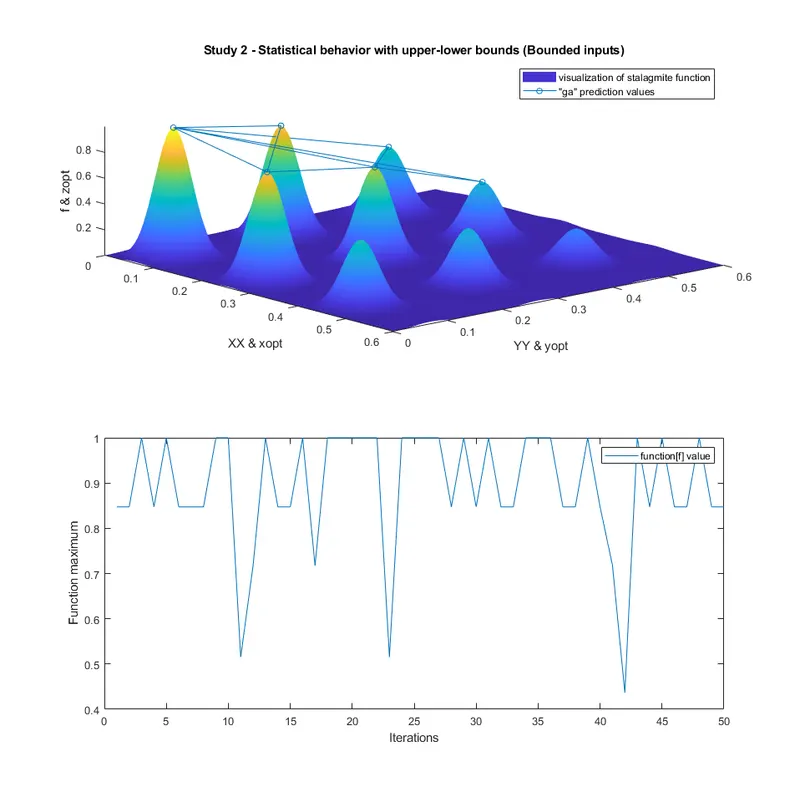
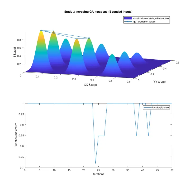
6. ERROR WHILE PROGRAMMING :
A. getting error "The surface Z must contain more than one row or column."?
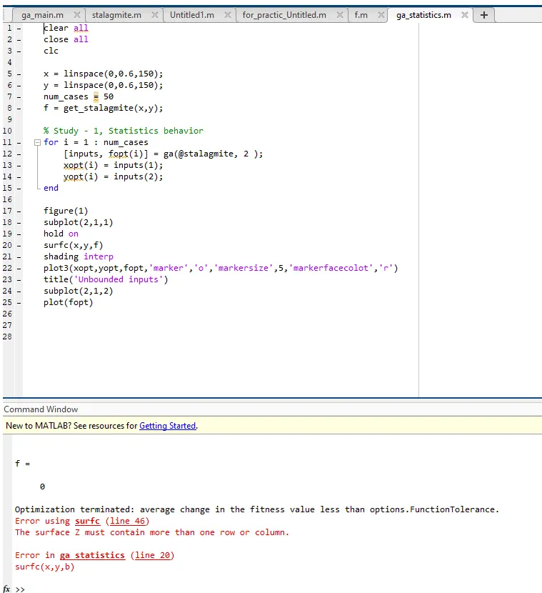
-- In this problem, I forgotten to include " f = get_stalagmite(x,y);" in " for loop."
B. getting fopt value to '0'zero
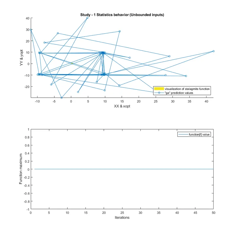
-- In this problem, there is a '-' sign missing in stalagmit function. beacause GA tends to find the minimum value of function and hence the possible minimum value for the set of positive values will be "0" and that's the reason I getting zero as an output.
7. CONCLUSION :
- Study-1 has no constraints, So every time it generates data with the random variable.
- Study-2 has upper-lower constraints, So now every time it generates data with accuracy arround 'globle maxima'.
- Study-3 has upper-lower constraints with population control. Using populationsize we Increasing 'ga' iteration. That providing 'ga' to more control to get accurate results. Here by increasing populationsize we will get maximum possible height of Stalagmite.
- Based on those three study we can understand how to control 'ga' 'optimization tool' in Matlab.
8. REFERENCE :