Project 2 - Rankine cycle Simulator
1. AIM : Create a Rankine Cycle Simulator using OCTAVE/MATLAB
2. GOVERNING EQUATIONS :
Here are some equations that are used at the end of cycle to calculate work, efficiency & more.
- Turbine work `W_T = h1-h2` `(frac{kJ}{kg})`
- Pump work `W_p = h4-h3` `(frac{kJ}{kg})`
- Net work done `W_"net" = W_T - W_p` `(frac{kJ}{kg})`
- Heat Addition `Q_"in" = h1 - h4` `(frac{kJ}{kg})`
- Heat Rejection `Q_"out" = h2 - h3` `(frac{kJ}{kg})`
- Thermal_Effi `eta_"th" = (frac{W_"net"}{Q_"in"})*100` `(%)`
- Specific steam consumption, ` SSC = frac{3600}{W_"net"}` `(frac{kJ}{kwh})`
- Back Work Ratio, `BWR = frac{W_p}{W_T}`
3. OBJECTIVES OF THE PROJECT :
Write a program in Matlab/Octave that do as per below:
- Calculate the state points of the Rankine Cycle based on user inputs
- Plot the corresponding T-s and h-s plots for the given set of inputs's results
- Calculate the "Net work output" & "Back work ratio
Here for User Input value is:
Turbine Inlet temperature = 400° C
Turbine Inlet Pressure = 30 bars
Turbine Outlet Pressure = 0.05 bars = Condenser Inlet Pressure
4. BODY OF THE CONTENT :
- INTRODUCTION :
A Brief Introduction about Rankine Cycle:
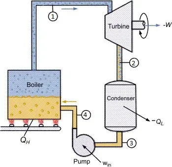
The Rankine Cycle is a mechanical cycle that is used to convert the pressure energy of steam into mechanical energy through steam turbines. The Rankine Cycle’s major components are a rotating steam turbine, a stationary condenser, a boiler pump and a boiler.
A boiler is used to heat the water for steam at the required pressure and temperature as per the turbine’s requirement for power generation. The turbine exhaust is directed to the radial or axial flow condenser for condensing the steam to condensate and recycled back to the boiler through boiler pumps for heating again.
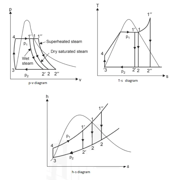
The Rankine cycle's p-v. T-s & h-s diagrams are shown. It comprises of the following processes:
Process 1-2 : Reversible adiabatic expansion in the turbine
Process 2-3 : Constant-pressure transfer of heat in the condenser
Process 3-4 : Reversible adiabatic pumping process in the feed pump
Process 4-1 : Constant-pressure transfer of heat in the boiler
- EXPLAINING LOGIC BEHIND MY CODE :
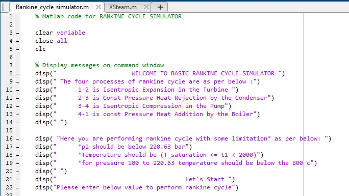
On the First Stage I wrote an Introduction message to display in the command window.
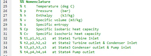
Then some Nomenclature was written.
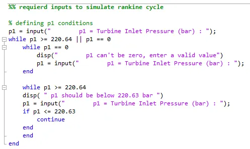
For User Input ,
Using a while loop Here I define p1 input.
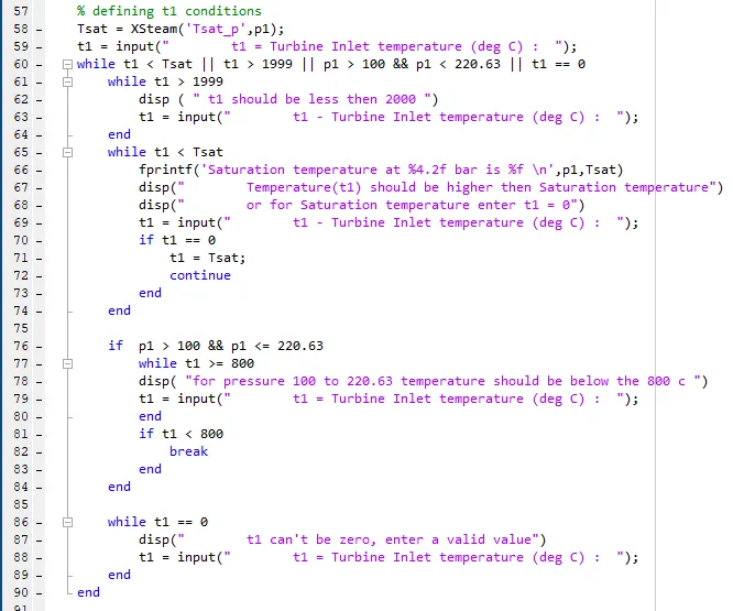
Then define t1 input value,
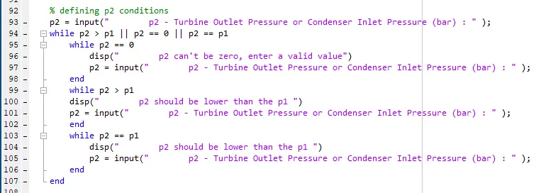
Then define the last input of p2 value.
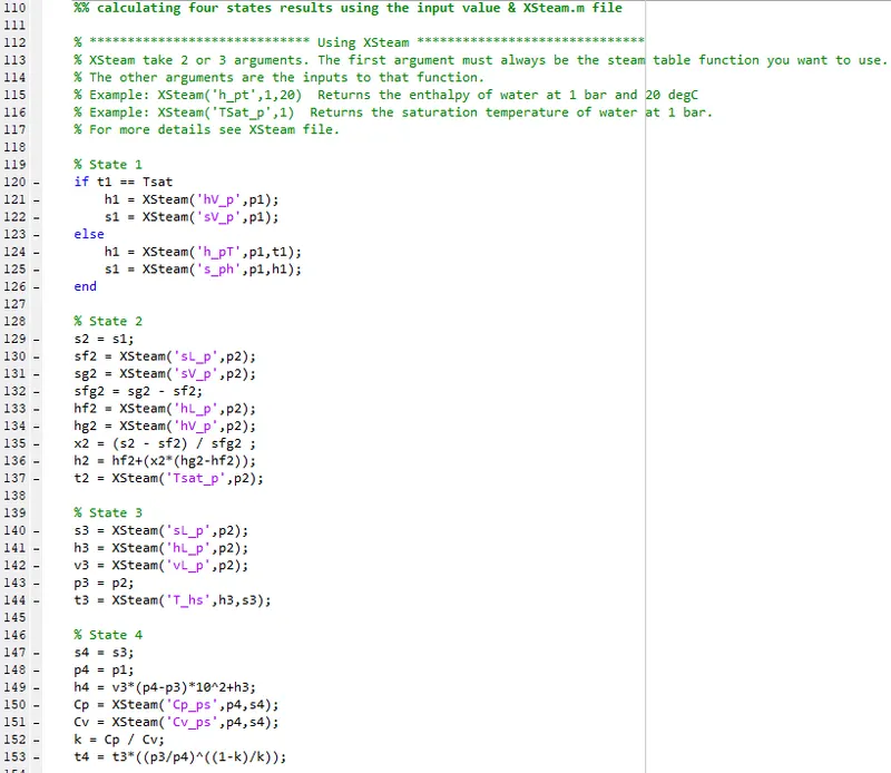
Now, As per user input data & XSteam file Calculating a pressure,temperature,entropy,enthalpy for different four states.
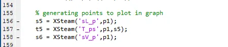
While calculating state points, some points are not included in the calculation but while plotting the result some extra points are required ,So calculating remaining points.
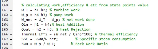
From the State points value calculating Final Results as shown above equations.
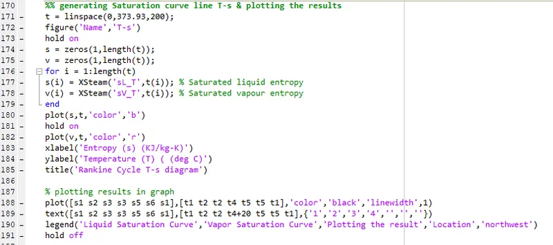
Now generating saturation curve for T-s diagram & plotting the four state points results.
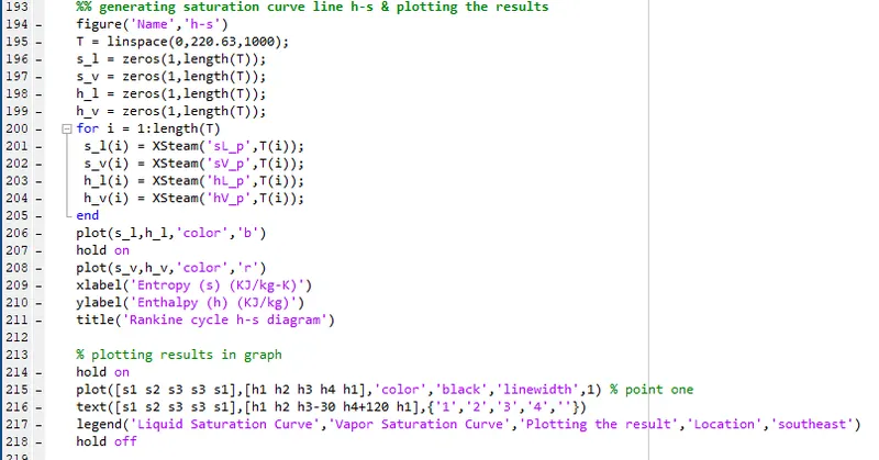
Now generating Saturation curve for h-s diagram & plotting the 4 state value.
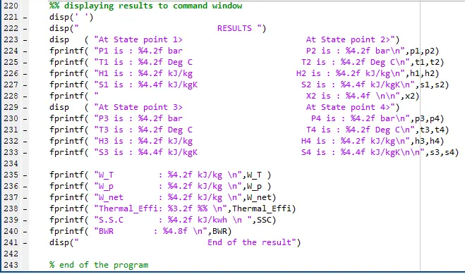
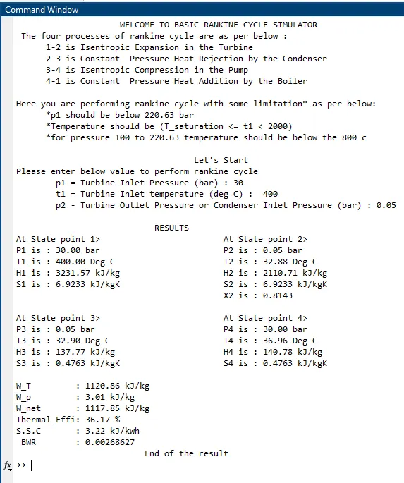
Finally , Displaying the All four state points & Work , Efficiency, S.S.C & BWR to the command window.
5. MATLAB code :
# INPUT :
% Matlab code for RANKINE CYCLE SIMULATOR

clear variable
close all
clc

% Display messages on command window
disp("                     WELCOME TO BASIC RANKINE CYCLE SIMULATOR ")
disp(" The four processes of rankine cycle are as per below :")
disp("      1-2 is Isentropic Expansion in the Turbine ")
disp("      2-3 is Constant  Pressure Heat Rejection by the Condenser")
disp("      3-4 is Isentropic Compression in the Pump")
disp("      4-1 is Constant  Pressure Heat Addition by the Boiler")
disp(" ")

disp( "Here you are performing rankine cycle with some limitation* as per below: ")
disp("      *p1 should be below 220.63 bar")
disp("      *Temperature should be (T_saturation <= t1 < 2000)")
disp("      *for pressure 100 to 220.63 temperature should be below the 800 c")
disp(" ")
disp("                                    Let's Start ")
disp("Please enter below value to perform rankine cycle")

%% Nomenclature
% t     Temperature (deg C)
% p	    Pressure    (bar)
% h	    Enthalpy    (kJ/kg)
% v	    Specific volume (m3/kg)
% s	    Specific entropy
% Cp	Specific isobaric heat capacity
% Cv	Specific isochoric heat capacity
% t1,p1,h1,s1   at State1 Turbine Inlet
% t2,p2,h2,s2   at State2 Turbine outlet & Condenser Inlet
% t3,p3,h3,s3   at State3 Condenser outlet & Pump inlet
% t4,p4,h4,s4   at State4 Pump outlet


%% required  inputs to simulate rankine cycle

% defining p1 conditions
p1 = input("        p1 = Turbine Inlet Pressure (bar) : ");
while p1 >= 220.64 || p1 == 0
    while p1 == 0
        disp("        p1 can't be zero, enter a valid value")
        p1 = input("        p1 = Turbine Inlet Pressure (bar) : ");
    end

    while p1 >= 220.64
    disp( " p1 should be below 220.63 bar ")
    p1 = input("        p1 = Turbine Inlet Pressure (bar) : ");
    if p1 <= 220.63
        continue
    end
    end
end

% defining t1 conditions
Tsat = XSteam('Tsat_p',p1);
t1 = input("        t1 = Turbine Inlet temperature (deg C) :  ");
while t1 < Tsat || t1 > 1999 || p1 > 100 && p1 < 220.63 || t1 == 0
    while t1 > 1999
        disp ( " t1 should be less then 2000 ")
        t1 = input("        t1 - Turbine Inlet temperature (deg C) :  ");
    end
    while t1 < Tsat
        fprintf('Saturation temperature at %4.2f bar is %f \n',p1,Tsat)
        disp("        Temperature(t1) should be higher then Saturation temperature")
        disp("        or for Saturation temperature enter t1 = 0")
        t1 = input("        t1 - Turbine Inlet temperature (deg C) :  ");
        if t1 == 0
            t1 = Tsat;
            continue
        end
    end

    if  p1 > 100 && p1 <= 220.63
        while t1 >= 800
        disp( "for pressure 100 to 220.63 temperature should be below the 800 c ")
        t1 = input("        t1 = Turbine Inlet temperature (deg C) :  ");
        end
        if t1 < 800
            break
        end
    end

    while t1 == 0
        disp("        t1 can't be zero, enter a valid value")
        t1 = input("        t1 = Turbine Inlet temperature (deg C) :  ");
    end
end

% defining p2 conditions
p2 = input("        p2 - Turbine Outlet Pressure or Condenser Inlet Pressure (bar) : " );
while p2 > p1 || p2 == 0 || p2 == p1
    while p2 == 0
        disp("        p2 can't be zero, enter a valid value")
        p2 = input("        p2 - Turbine Outlet Pressure or Condenser Inlet Pressure (bar) : " );
    end
    while p2 > p1
    disp("        p2 should be lower than the p1 ")
    p2 = input("        p2 - Turbine Outlet Pressure or Condenser Inlet Pressure (bar) : " );
    end
    while p2 == p1
        disp("        p2 should be lower than the p1 ")
        p2 = input("        p2 - Turbine Outlet Pressure or Condenser Inlet Pressure (bar) : " );
    end
end


%% calculating four states results using the input value & XSteam.m file

% ***************************** Using XSteam ******************************
% XSteam take 2 or 3 arguments. The first argument must always be the steam table function you want to use.
% The other arguments are the inputs to that function.
% Example: XSteam('h_pt',1,20)  Returns the enthalpy of water at 1 bar and 20 degC
% Example: XSteam('TSat_p',1)  Returns the saturation temperature of water at 1 bar.
% For more details see XSteam file.

% State 1
if t1 == Tsat
    h1 = XSteam('hV_p',p1);
    s1 = XSteam('sV_p',p1);
else
    h1 = XSteam('h_pT',p1,t1);
    s1 = XSteam('s_ph',p1,h1);
end

% State 2
s2 = s1;
sf2 = XSteam('sL_p',p2);
sg2 = XSteam('sV_p',p2);
sfg2 = sg2 - sf2;
hf2 = XSteam('hL_p',p2);
hg2 = XSteam('hV_p',p2);
x2 = (s2 - sf2) / sfg2 ;
h2 = hf2+(x2*(hg2-hf2));
t2 = XSteam('Tsat_p',p2);

% State 3
s3 = XSteam('sL_p',p2);
h3 = XSteam('hL_p',p2);
v3 = XSteam('vL_p',p2);
p3 = p2;
t3 = XSteam('T_hs',h3,s3);

% State 4
s4 = s3;
p4 = p1;
h4 = v3*(p4-p3)*10^2+h3;
Cp = XSteam('Cp_ps',p4,s4);
Cv = XSteam('Cv_ps',p4,s4);
k = Cp / Cv;
t4 = t3*((p3/p4)^((1-k)/k));

% generating points to plot in graph
s5 = XSteam('sL_p',p1);
t5 = XSteam('T_ps',p1,s5);
s6 = XSteam('sV_p',p1);

% calculating work,efficiency & etc from state points value
W_T = h1-h2; % turbine work
W_p = h4-h3; % pump work
W_net = W_T - W_p; % net work done
Qin = h1 - h4;% heat Addition
Qout = h2 - h3; % heat Rejection
Thermal_Effi = (W_net / Qin)*100; % thermal efficiency
SSC = 3600/W_net;        % Specific steam consumption
BWR = W_p / W_T;       % Back Work Ratio

%% generating Saturation curve line T-s & plotting the results
t = linspace(0,373.93,200);
figure('Name','T-s')
hold on
s = zeros(1,length(t));
v = zeros(1,length(t));
for i = 1:length(t)
s(i) = XSteam('sL_T',t(i)); % Saturated liquid entropy
v(i) = XSteam('sV_T',t(i)); % Saturated vapour entropy
end
plot(s,t,'color','b')
hold on
plot(v,t,'color','r')
xlabel('Entropy (s) (KJ/kg-K)')
ylabel('Temperature (T) ( (deg C)')
title('Rankine Cycle T-s diagram')

% plotting results in graph
plot([s1 s2 s3 s3 s5 s6 s1],[t1 t2 t2 t4 t5 t5 t1],'color','black','linewidth',1)
text([s1 s2 s3 s3 s5 s6 s1],[t1 t2 t2 t4+20 t5 t5 t1],{'1','2','3','4','','',''})
legend('Liquid Saturation Curve','Vapor Saturation Curve','Plotting the result','Location','northwest')
hold off

%% generating saturation curve line h-s & plotting the results
figure('Name','h-s')
T = linspace(0,220.63,1000);
s_l = zeros(1,length(T));
s_v = zeros(1,length(T));
h_l = zeros(1,length(T));
h_v = zeros(1,length(T));
for i = 1:length(T)
 s_l(i) = XSteam('sL_p',T(i));
 s_v(i) = XSteam('sV_p',T(i));
 h_l(i) = XSteam('hL_p',T(i));
 h_v(i) = XSteam('hV_p',T(i));
end
plot(s_l,h_l,'color','b')
hold on
plot(s_v,h_v,'color','r')
xlabel('Entropy (s) (KJ/kg-K)')
ylabel('Enthalpy (h) (KJ/kg)')
title('Rankine cycle h-s diagram')

% plotting results in graph
hold on
plot([s1 s2 s3 s3 s1],[h1 h2 h3 h4 h1],'color','black','linewidth',1) % point one
text([s1 s2 s3 s3 s1],[h1 h2 h3-30 h4+120 h1],{'1','2','3','4',''})
legend('Liquid Saturation Curve','Vapor Saturation Curve','Plotting the result','Location','southeast')
hold off

%% displaying results to command window
disp(' ')
disp("                            RESULTS ")
disp   ( "At State point 1>                         At State point 2>")
fprintf( "P1 is : %4.2f bar                         P2 is : %4.2f bar\n",p1,p2)
fprintf( "T1 is : %4.2f Deg C                      T2 is : %4.2f Deg C\n",t1,t2)
fprintf( "H1 is : %4.2f kJ/kg                     H2 is : %4.2f kJ/kg\n",h1,h2)
fprintf( "S1 is : %4.4f kJ/kgK                     S2 is : %4.4f kJ/kgK\n",s1,s2)
fprintf( "                                          X2 is : %4.4f \n\n",x2)
disp   ( "At State point 3>                         At State point 4>")
fprintf( "P3 is : %4.2f bar                          P4 is : %4.2f bar\n",p3,p4)
fprintf( "T3 is : %4.2f Deg C                       T4 is : %4.2f Deg C\n",t3,t4)
fprintf( "H3 is : %4.2f kJ/kg                      H4 is : %4.2f kJ/kg\n",h3,h4)
fprintf( "S3 is : %4.4f kJ/kgK                     S4 is : %4.4f kJ/kgK\n\n",s3,s4)

fprintf( "W_T         : %4.2f kJ/kg \n",W_T )
fprintf( "W_p         : %4.2f kJ/kg \n",W_p )
fprintf( "W_net       : %4.2f kJ/kg \n",W_net)
fprintf( "Thermal_Effi: %3.2f %% \n",Thermal_Effi)
fprintf( "S.S.C       : %4.2f kJ/kwh \n ",SSC)
fprintf( "BWR        : %4.8f \n",BWR)
disp("                          End of the result")

% end of the program
# OUTPUT :
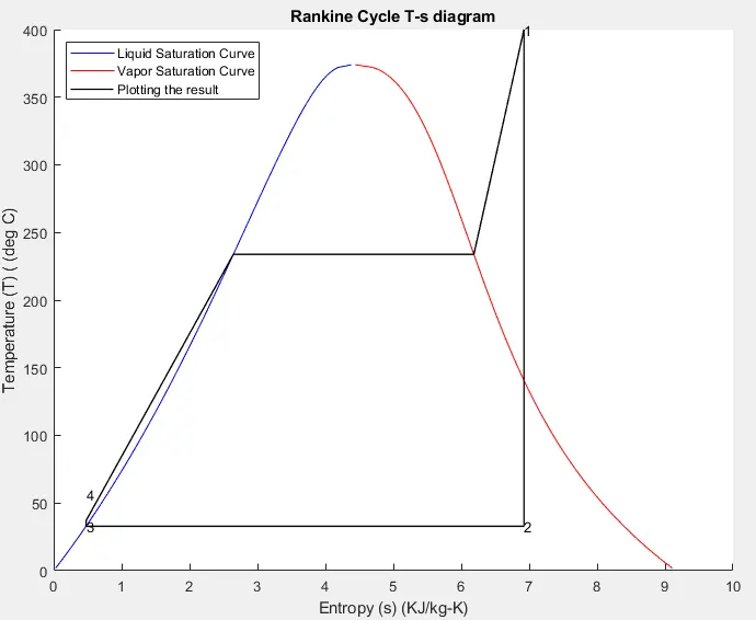
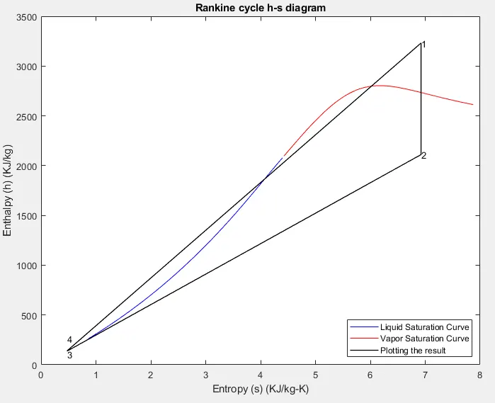
Command window output as per below,
- Errors faced while programming :
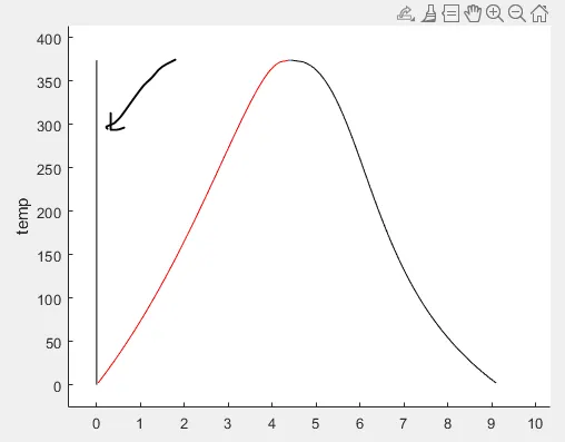
while plotting the curve this vertical line is coming,
it does happen because I created 200x200 matrix,
s = zeros(length(t));
v = zeros(length(t));
instead of only to create a row matrix.
like this
s = zeros(1,length(t));
v = zeros(1,length(t));
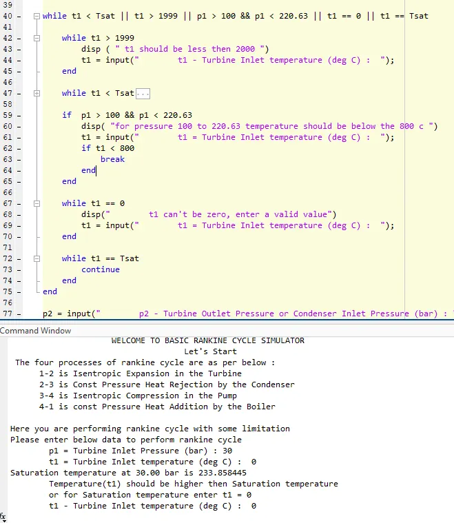
On entering t1 = 0 it stops on that stage, not going on to the next stage?
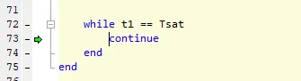
Then using a debugging process I find out that the command is stik at this line as shown above.
Then I found out that, This while loop " t1 == Tsat" was useless so I removed that one.
While Coding ,This type of Such condition does occur many time , But using debugging process I solve that very well.
6. CONCLUSION:
From this project I learn how to call data from different files. And How can I constrain an output or input of some value as per required.
Also, I learn that there is something wrong in code and how to find out and solve that issue.
- REFERENCES / literature / online material :